

Introduction
Motivation and Objectives
Methodology
Results
Wellbore configuration and fluid circulation
Simulation results of base scenario
Simulation results of scenario 1 and 2
Features captured by multi-dimensional simulations
Conclusions
Introduction
Cementing job is a process of injecting and placing cement to the annular space between casing and tubing. The most important function of cementing job is to provide zonal isolation, that is, isolating geological formations from the well such that the hydrocarbon fluids could be produced from the productive layers efficiently (Mitchell and Wedelich, 1989). Cementing job also supports the vertical and radial loads applied on the casing string and prevents corrosion of casing (Nelson and Guillot, 2006). Accurately predicting temperature profile, which changes with time, during fluid circulation is important because (i) higher temperatures tend to decrease the setting time (When cement is mixed with water, it hydrates and makes cement paste. This paste can be moulded into any desired shape due to its plasticity. Within this time cement continues with reacting water and slowly cement starts losing its plasticity and set harden. This complete cycle is called Setting time of cement (Dillenbeck and Mombourquette, 2001). The time to which cement can be moulded in any desired shape without losing its strength is called initial setting time of cement, while the time at which cement completely loses its plasticity and becomes hard is called final setting time of cement. The consequences of not achieving the correct setting time is significant because (i) the costs of drilling operation and well completion can be expensive (Bittleston, 1990) and (ii) even more importantly, such a delay in cement setting time can allow the flow of gas or water from shallow overpressured formations, potentially leading to erosion and catastrophic failure of the entire well (Calvert and Griffin, 1998).
The American Petroleum institute (API) has developed temperature correlations to estimate circulating temperatures for cementing job. Those correlations (API RP10B) are somewhat simplified and based on true vertical depth (TVD) and geothermal temperature gradient. While the correlations, originally intended for on-shore wells, provide useful and reasonable guidelines, its applicability for offshore wells is still challenging, especially for some wells drilled in deep water (Chen and Xie, 2015).
Chen and Novotny (2003) mentioned the wellbore temperature is mainly affected by parameters such as cement thickening time (or, wait on cementing), cement compressive strength development, fluid rheology, and fluid loss during cementing job. Wang and Dai (2018) added additional parameters of importance such as circulation time, circulation rate, fluid inlet temperature, geothermal temperature, wellbore geometry (dimensions and deviations), fluid densities and thermal properties, water depth and current for offshore wells.
To achieve a successful cement job design, three basic categories of parameters were suggested (Nelson and Guillot, 2006): well depth and well configuration, wellbore environment (fluid distribution, open-hole and cased-hole sections, formation pore and fracturing pressures), and temperature data of surrounding areas. These parameters are used to determine the bottomhole circulating temperature (BHCT), bottomhole static temperature (BHST), and temperature differential between the bottom and top of the cement column. Examples to estimate BHCT are shown in API Spec 10 and in computer simulators, the latter of which has been widely used to model complicated situations where the physics of heat transfer and dynamic conditions need to be taken into consideration (Goodman et al., 1988; Karstad and Aadnoy,1999).
For example, Calvert and Griffin (1998) utilized two simulators: the first is a one-dimensional simulator that is first introduced by Guillot et al. (1993) and Bittleston (1990), and the second is an improved two-dimensional model to compare the circulating temperature profile with API prediction. The results from the simulation of offshore wells with deep water depths of 7,200 ft showed that the API correlations may not be applicable to deep water wells because the API uses an average temperature gradient from surface to the bottom of the well to determine the static temperature, but the offshore deepwater wells have large variations of sea temperature gradient which can not be represented by one single average temperature gradient (Guzman et al., 2018). There are numerous other computer simulation studies in the literature that take advantage of computational fluid dynamics (CFD) modeling since then. They combine complicated fluid mechanics problems with heat transfer (Kabinoff et al., 1992).
Motivation and Objectives
This study is motivated by Chen and Novotny (2003) and Wang and Dai (2018).
Chen and Novotny (2003) developed a one-dimensional in-house numerical simulator by using a finite difference method (FDM) to predict temperature profile in wellbore during fluid circulation in onshore and offshore wells. When compared with their own field test measurements (temperature as a function of time at three different locations) during the circulation of seawater, the study showed that the offshore wells are much more difficult to predict than the onshore wells.
Wang and Dai (2018) re-visited the study from Chen and Novotny (2003) by using a commercial software CEMPRO, specialized for cementing job, solving for coupled fluid mechanics and heat transfer. They predicted temperature profile along the wellbore, similar to Chen and Novotny (2003).
These and other similar studies in the literature have common limitations. Although computationally convenient and time efficient for practical applications, the one- dimensional nature of simulations fails to show (i) the velocity profile in axial directions within the tubing and annulus areas and (ii) the complicated behavior near the fluid interface (where the displacing fluid interacts with the displaced fluid) and at the bottom hole (where the fluid faces a sudden change in flow direction within a narrow conduit).
Therefore, the objective of this study is to (i) evaluate multi-dimensional transient simulations for the prediction of temperature profile during cementing job and (ii) understand the possible benefits to guide widely used one-dimensional simulations. ANSYS Fluent is selected as a multi-dimensional transient CFD tool in this study and the offshore field case studied in Chen and Novotny (2003) and Wang and Dai (2018) is used as a base scenario. In addition to circulating seawater into the well originally filled with seawater (base scenario), this study investigates two other scenarios (scenario 1 and 2) when seawater is circulated into the well filled with drilling mud and when drilling mud is circulated into the well filled with seawater, respectively.
Methodology
There are three major governing equations associated with transient wellbore temperature simulations - mass conservation equation, momentum conservation equation and energy balance equation. While the mass and momentum conservation equations deal with the transport of involving phases, the energy balance equation solves for heat conduction and convection as well as sink/source terms. The system consists of fluids inside drill pipe, drill pipe wall, fluids in the annulus between drill pipe and casing, casing wall and the surrounding formation. Heat conduction is considered in the formations, drill pipe wall, and casing wall, whereas heat convection is considered through the fluids in drill pipe, and in the annulus between drill pipe and casing. In the case of offshore wells, the annulus space between drill pipe and riser must be taken into consideration.
The partial differential equation for mass conservation equation for 2D axisymmetric geometries can be written as follows:
| $$\frac{\partial\rho}{\partial t}+\frac{\displaystyle\partial}{\displaystyle\partial x}(\rho v_x)+\frac{\displaystyle\partial}{\displaystyle\partial r}(\rho v_r)+\frac{\rho v_r}r=S_m$$ | (1) |
where and represent the time and phase density. In addition, is the axial coordinate, is the radial coordinate, is the axial velocity, and is the radial velocity. Eq. (1) is valid for incompressible as well as compressible flows. The source is the mass added to the continuous phase from the dispersed second phase, if present, and any user-defined sources.
Conservation of momentum in an inertial reference frame is described below:
| $$\frac\partial{\partial t}(\rho\overrightarrow v)+\nabla\cdot(\rho\overrightarrow v\overrightarrow v)=-\nabla p+\nabla\cdot(\overline\tau)+\rho\overrightarrow g+\overrightarrow F$$ | (2) |
where is the static pressure, is the velocity vector, is the stress tensor, and and are the gravitational body force and external body forces, respectively. may also contain other model-dependent source terms such as porous-media.
The stress tensor is given by
| $$\overline{\overline\tau}=\mu\left\lceil(\triangle\overrightarrow v+\triangle\overrightarrow v^T)-\frac23\nabla\cdot\overrightarrow vI\right\rceil$$ | (3) |
where is the phase viscosity and is the unit tensor. Note that the second term on the right-hand side is the effect of volume dilation.
For 2D axisymmetric geometries, the axial and radial momentum conservation equations are given by:
and
where
| $$\nabla\cdot\overrightarrow v=\frac{\displaystyle\partial v_r}{\displaystyle\partial x}+\frac{\displaystyle\partial v_r}{\displaystyle\partial r}+\frac{\displaystyle v_r}{\displaystyle r}$$ | (6) |
and is the swirl velocity.
The partial differential equation for energy balance can be written as follows:
where is the effective conductivity, is the overall energy (internal energy and kinetic energy combined), is the temperature, is the enthalpy of species j and is the diffusion flux of species j. The first three terms on the right-hand side of Eq. (7) represent energy transfer due to conduction, species diffusion, and viscous dissipation, respectively. includes the heat from chemical reaction and any other volumetric heat sources.
ANSYS Fluent solves these governing equations by using finite difference methods. Briefly describing, Fluent is a commercial software which contains the broad physical modeling capabilities needed to model flow, heat transfer and other industrial applications including drilling and completion. Fluent can also be used for simulating cementing job to calculate cementing displacement efficiency by using volume of fluid (VOF) model to capture volume fraction of each phase in fluid domain (Merlo et al., 1995). The VOF model can model two or more immiscible fluids by solving a single set of momentum equations and tracking the volume fraction of each of the fluids throughout the domain (Fluent Theory Guide, 2016). In addition, the VOF method utilizes a single energy equation for the entire system, which is very useful to simulate interface resolved physical problems such as hydrodynamics. Those problems with heat and mass transfer phenomena can also be simulated (Erge et al., 2015).
Results
Wellbore configuration and fluid circulation
The base scenario borrows well configuration from Chen and Novotny (2003) for comparison and validation, as schematically shown in Fig. 1. It is a vertical offshore well with water depth 3,780 ft and total depth is 5,721 ft. The casing has 20 in. OD and 19 in. ID, while the drill pipe has 5 in. OD and 4.276 in. ID. Outside the casing, a radial distance of 10 ft of geological formation is included as a part of the system. There is a 0.1 ft gap vertically between drill pipe bottom and casing bottom that allows fluid to flow from drill pipe to annulus. There are three temperature gauges installed to monitor temperature variations: at the wellbore (z = 5,721 ft inside drill pipe), in the middle of the well (z = 4,786 ft in the annulus) and at the top of the well (z = 0 ft in the annulus)
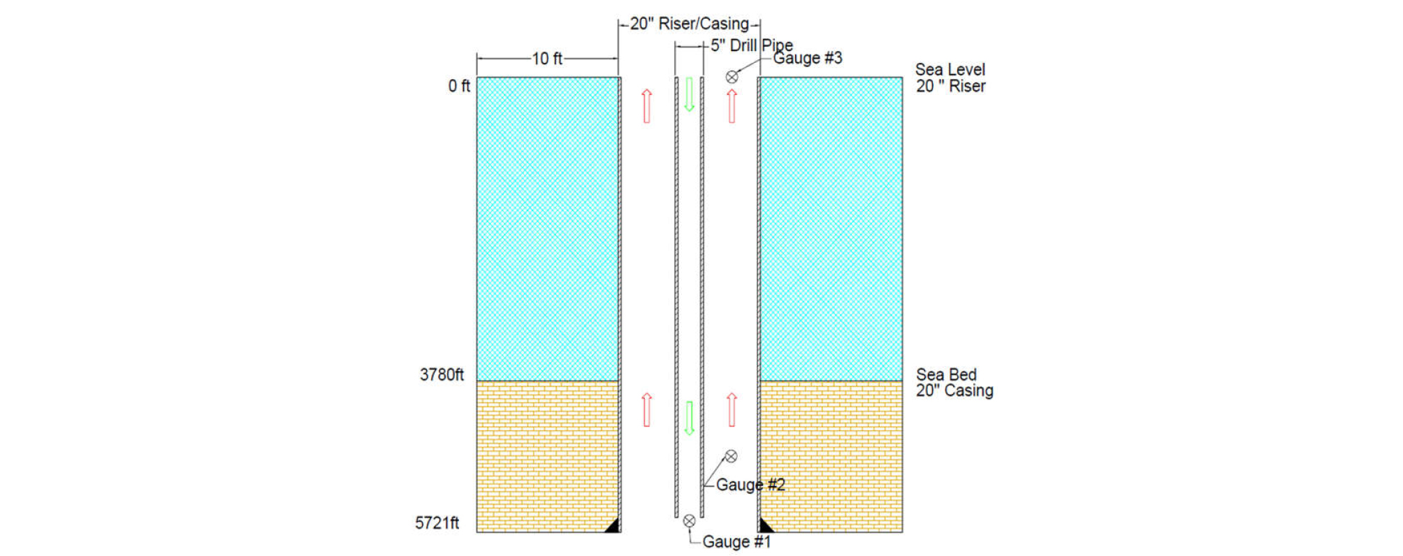
Fig. 2. shows how the system is discretized for numerical calculations. Along the radial direction, the formation consists of 39 grids, while the drill pipe and annulus spaces consist of 7 grids and 12 grids radially, respectively. Along the vertical direction, each grid has a length of 1.4 ft with about 4,100 grids except the bottom hole area where much finer grid system is applied (this is needed for accuracy of calculations as well as the stability of numerical calculations). Casing and drill pipe walls consist of 3 grids.

The model requires the properties of two fluids (seawater and drilling mud) and two solid materials (drill pipe/casing and formation) as shown in Table 1 and Table 2. Initially (t = 0), the well (both drill pipe and annulus) is occupied by seawater and another seawater of the same properties is injected as a base scenario. Scenario 1 and 2 are further considered for ‘seawater injection into the well initially filled with drilling mud’ and ‘drilling mud injection into the well initially filled with seawater’. Seawater is approximated by Newtonian fluid and drilling mud is modeled by yield power-law fluid (with yield stress (ty), consistency index (K), and shear-thinning parameter (n)). It is assumed that all fluids are incompressible and there are no phase changes. Because the well is vertical and axisymmetric, this three-dimensional problem can be simplified and solved as a two-dimensional problem.
Table 1. Input data for fluid properties
Table 2. Input data for solid properties
| Material list | Density, kg/m3 | Thermal Conductivity, w/(m°C) | Specific Heat, J/(kg°C) |
| Casing and Drill Pipe | 7,848.8 | 45.0 | 879.2 |
| Surrounding Formation | 2,240.8 | 1.59 | 1,256.0 |
The injection rate (Qin) is 10 bpm from t = 0 to 10 minutes, and 39.66 bpm for t = 10 to 60 minutes, as shown in the pumping schedule of Table 3. For the first 10 minutes, the low injection rate (Qin = 10 bpm) is designated to displace the fluid in drill pipe, and for the other 50 minutes, the high injection rate (Qin = 39.66 bpm) is designed to displace the fluid in annulus. As a result, the entire 60 minutes injection period is designated to displace roughly all of the fluids in the well (both drill pipe and annulus). The injected fluid is assumed to have the same temperature as surface temperature (Ts),thatis,Ts=77°F. The seawater and formation have vertical temperature gradients of dTw/dz and dTf/dz, respectively, which vary with depth (z) (i.e., does not have to be linear), the details of which are shown in the next section.
Table 3. Input data for pumping schedule in simulation
| Fluid | Liquid volume injected (bbl) | Injection rate Qin (bpm) | Stage Time (min) | Cumulative Time (min) |
| Seawater or Mud | 100 | 10.00 | 10 | 0 to 10 |
| Seawater or Mud | 1,983 | 39.66 | 50 | 10 to 60 |
Simulations have been performed with the inlet condition specified by the injection rate (Qin) and the outlet condition is specified as a fixed pressure (i.e., atmospheric pressure).
Simulation results of base scenario
Base scenario accounts for the injection of seawater into the well originally occupied by seawater. Fig. 3. shows how temperature profile (T vs. z) changes with time (t = 10, 20, 40 and 60 minutes) in addition to the initial temperature profile. The results look complicated because of the effects from the seawater temperature gradient as well as formation temperature gradient - T decreases with z in the seawater, while T increases with z within the formation. With time, the temperature profile approaches a steady-state response, and the temperature wave moves concurrently with flow direction (i.e., from the top to the bottom on the drill pipe side; from the bottom to the top on the annulus side).

The results at three different measurement depths are shown in Figs. 4. through 6 at z = 5,721 ft (within drill pipe), 4,786 ft (within the annulus), and 0 ft (within the annulus), respectively. There are a few interesting aspects observed. First of all, thinking of the fact that the actual temperature measurements are reported to have a few to several minutes time lag, those one-dimensional simulations from Chen and Novotny (2003) and Wang and Dai (2018) capture the trend reasonably well. Second, the two- dimensional simulation results in this study can produce similar responses but, in all three locations, it takes longer time to reach the same level of changes. This is because simulation in multi-dimensional space allows temperature variations in radial direction which contributes to more time for heat transfer. Last, temperature variation in axial direction (center vs. edge (near the wall) in Fig. 4; center vs. inner edge (near the drill pipe wall) vs. outer edge (near the casing wall) in Figs. 5 and 6) does not seem to be significant (less than 1oF), but it may take as much as several minutes for heat transfer to overcome the temperature gap.


Simulation results of scenario 1 and 2
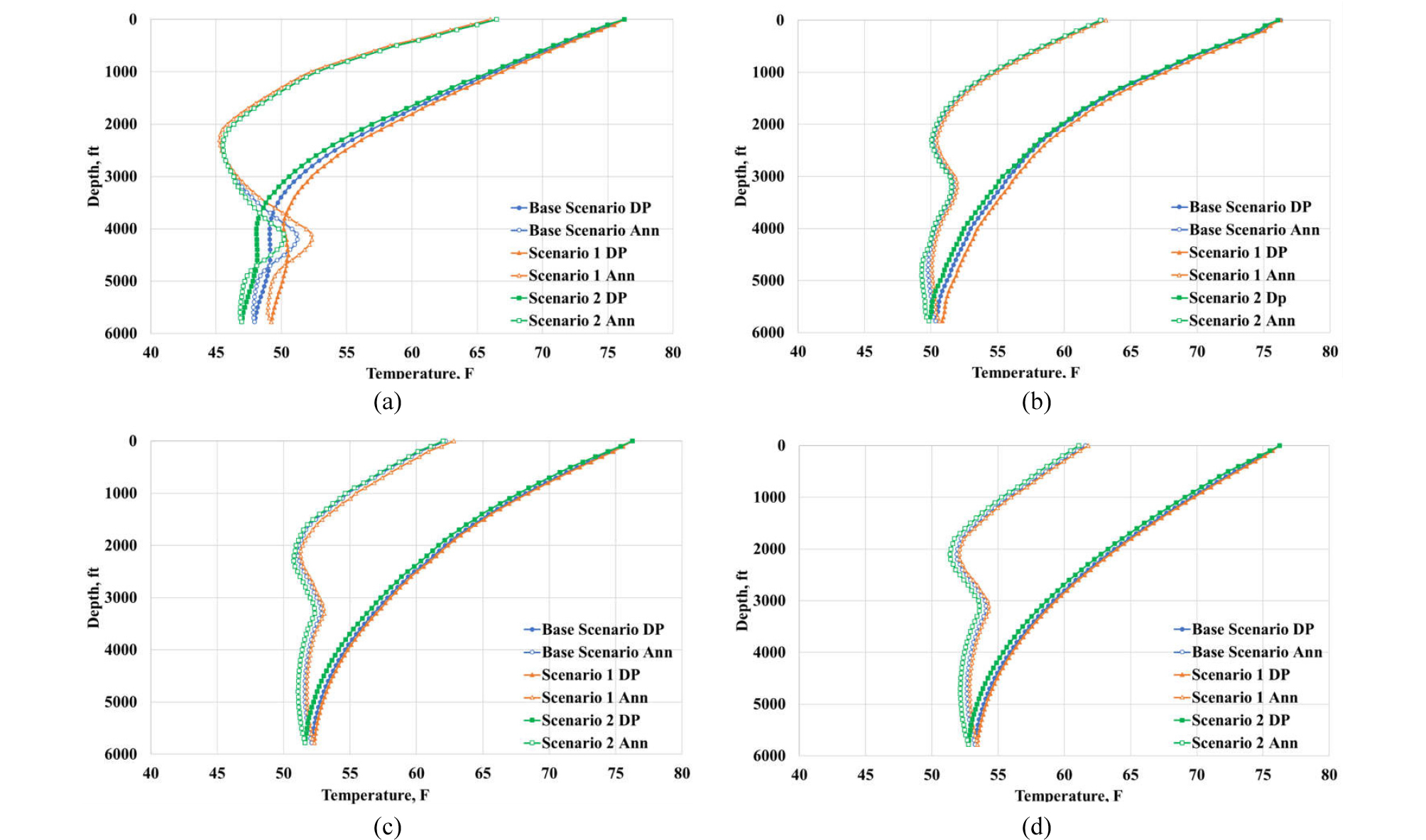
Fig. 7(a) and 7(b) show the temperature profiles as a function of time for scenario 1 and 2, respectively. The comparison with base scenario shows that the temperature profiles follow roughly the same trend, that is, the temperature wave travels concurrently with the flow direction. Also, similarly, the temperature profiles approach the steady-state response as well.
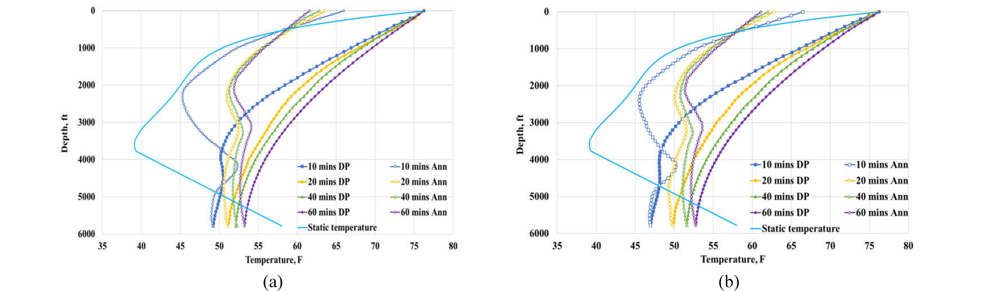
Fig. 8(a) to 8(d) provides a closer comparison at t = 10, 20, 40, and 60 minutes, respectively, for all three scenarios. Two interesting aspects are observed. First, the gap in temperature profiles between different scenarios is larger in earlier time (eg. t = 10 minutes) and rapidly narrows down with time approaching the steady-state response. And second, because of high thermal conductivity of drilling mud compared to seawater (cf. Table 1), the temperature profile of scenario 1 (i.e., seawater injection into the well with mud) changes more rapidly than that of base scenario, and therefore the profile of scenario 1 sits on the right-hand side of the base scenario. On the contrary, the opposite happens for scenario 2 because of the similar reasons.
Features captured by multi-dimensional simulations
One way to check how multi-dimensional simulations differ from 1D simulations is to compare velocity profiles. For each of three scenarios (base scenario, scenario 1, and scenario 2), Figs. 9 and 10 present velocity vectors at t = 60 minutes (at the end of process), all on the same scale, at the vertical depths of z = 3,000 ft (middle of the well) and z = 5,721 ft (about 10 ft interval at the bottom hole), respectively
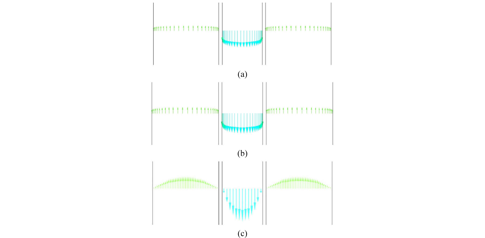
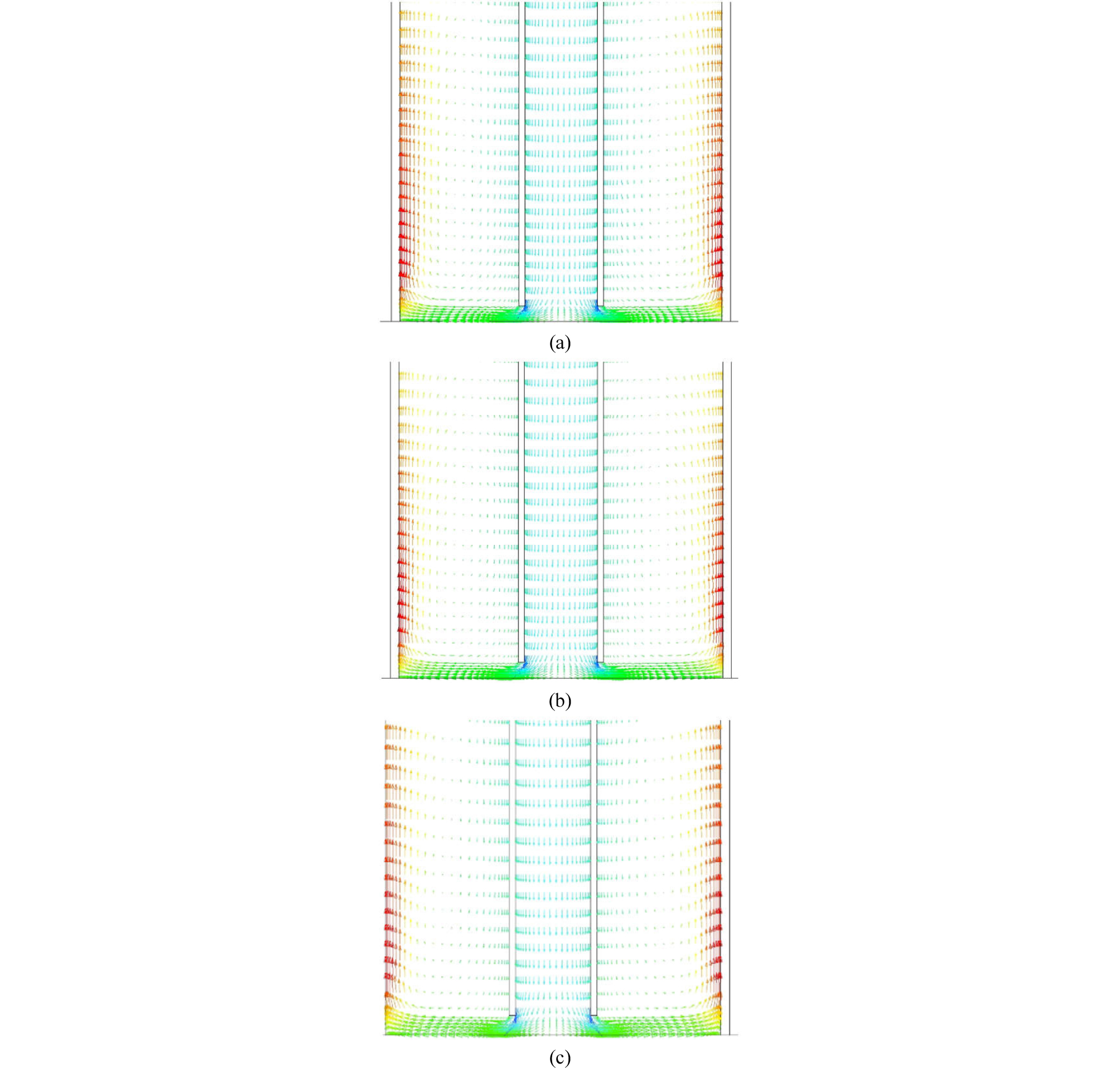
A few interesting observations can be made. First, even if the initial conditions are different, base scenario and scenario 1 show almost identical results at t = 60 minutes, as shown in Fig. 9(a) and 9(b) as well as Fig. 10(a) and 10(b), because of the same seawater injection replacing existing fluids. Second, scenario 2 with mud injection has a distinctly different velocity profile because of its shear thinning rheology and higher density compared with seawater (Table 1). Third, the average velocity in the drill pipe is much higher (as illustrated by longer arrows) than that in the annulus in all scenarios because of smaller cross-sectional area. Finally, the velocity vectors at the bottom hole in all three scenarios (Fig. 10) show much more complicated behaviors that 1D simulations cannot capture – rather than the displacing fluids migrate upward through the annulus from the bottom hole in a piston-like manner (as 1D simulation does), the fluids coming out of the pipe tend to flow towards the outer edge of the annulus due to momentum. Such a tendency is stronger in scenario 2 (Fig. 10(c)), as represented by longer arrows near the outer edge, because of the higher density of injected fluid (i.e., mud).
The tendency can be investigated further by tracking the movement of injected fluids along the well, as shown by Figs. 11 through 13 for base scenario, scenario 1 and scenario 2, respectively. In all figures, the first shows the movement of injected fluid when it is in the middle of the pipe (t = 5 minutes; z = 2,800 to 2,810 ft), while the second and third show when it is flowing into the annulus at the bottom hole (between t = 10 and 11 minutes; z = 5,711 to 5,721 ft). The last one shows the results at t = 60 minutes at the bottom hole (z = 5,711 to 5,721 ft).
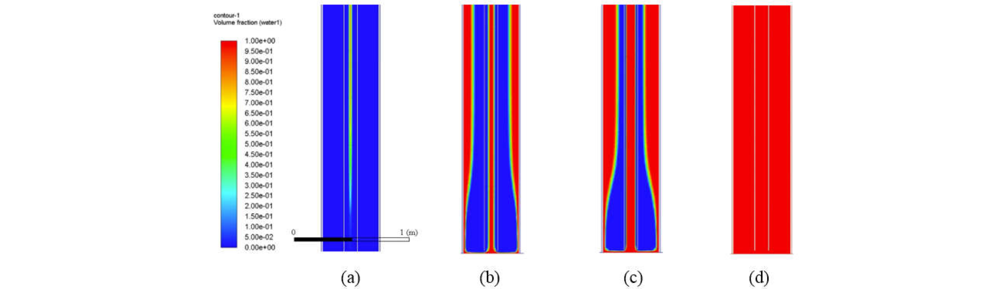
Fig. 11.
Volume fraction of injected seawater for base scenario: (a) t = 5, (b) t = 10.2, (c) t = 10.3 minutes, and (d) t = 30 minutes ((a) showing the middle of the well (z = 2,800 to 2,810 ft), while (b) through (d) showing the bottom of the well (z = 5,711 to 5,721 ft)). (The scale on the left shows the volume fraction from 0 to 1.).
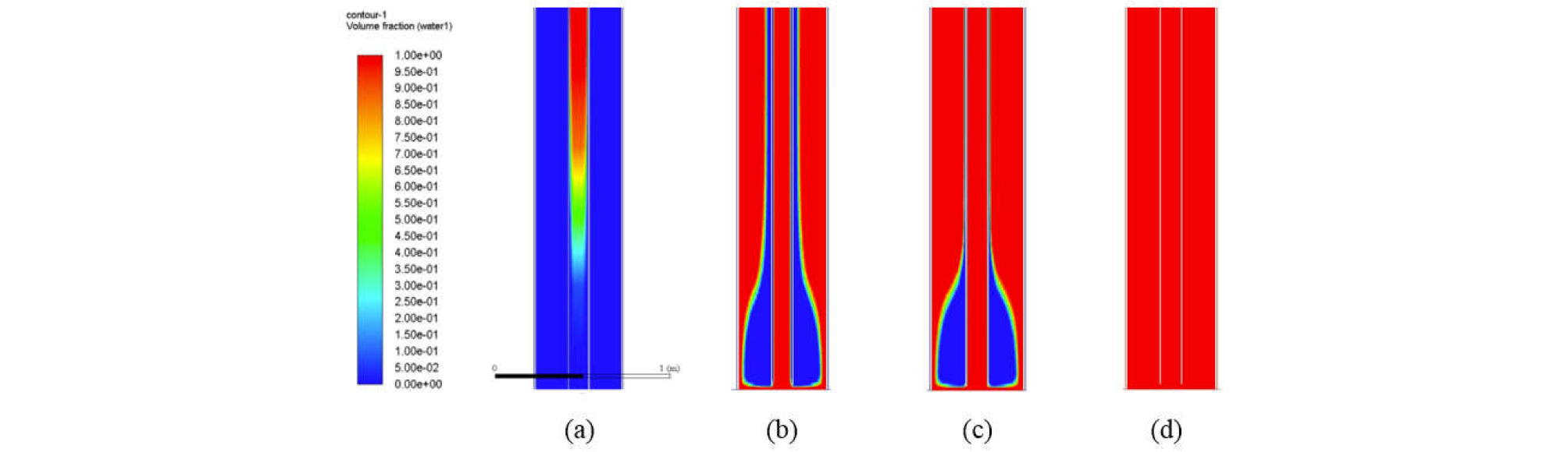
Fig. 12.
Volume fraction of injected seawater for scenario 1: (a) t = 5, (b) t = 10.5, (c) t = 11, and (d) t = 30 minutes ((a) showing the middle of the well (z = 2,800 to 2,810 ft), while (b) through (d) showing the bottom of the well (z = 5,711 to 5,721 ft)). (The scale on the left shows the volume fraction from 0 to 1.).
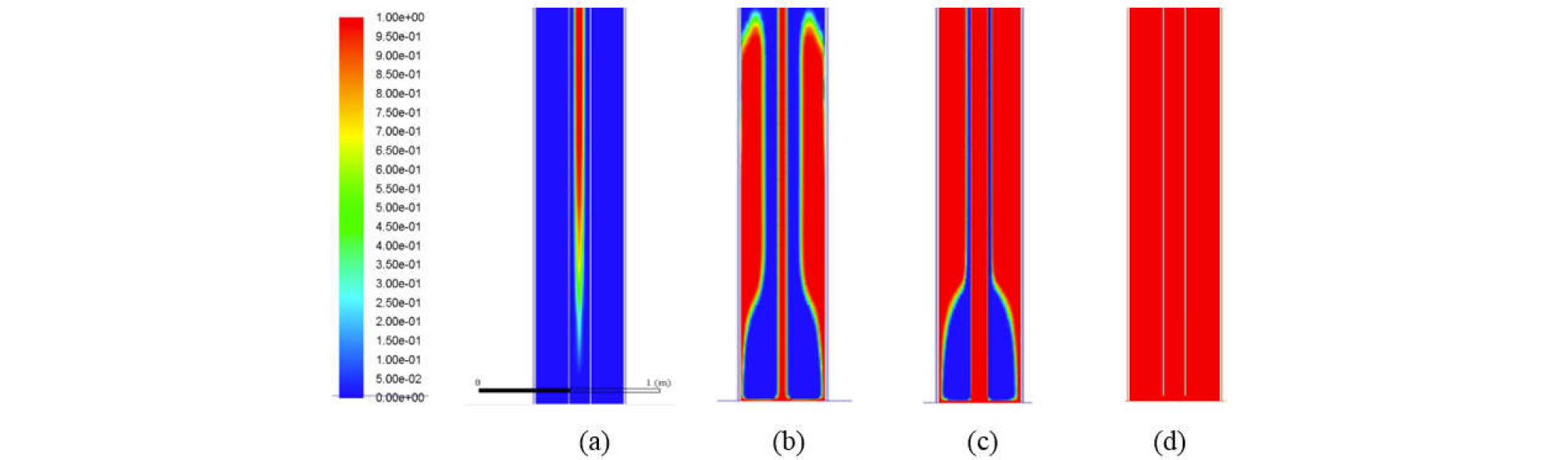
Fig. 13.
Volume fraction of injected drilling mud for scenario 2: (a) t = 5, (b) t = 10.5, (c) t = 11, and (d) t = 30 minutes ((a) showing the middle of the well (z = 2,800 to 2,810 ft), while (b) through (d) showing the bottom of the well (z = 5,711 to 5,721 ft)). (The scale on the left shows the volume fraction from 0 to 1.).
Figs. 11 through 13 indicate that the heat transfer problems based on 1D simulations can go very wrong, because they assume the movement of injected fluid marching from the bottom to the top in the annulus. The simulation results in all three scenarios demonstrate, however, that the injected fluid is stripping off the existing fluid from the outer edge to the inner edge of the annulus near the bottom hole. This difference can make a significant delay in heat transfer, and such a behavior partly explains why it takes longer for multi-dimensional simulation as shown in Figs. 4 through 6.
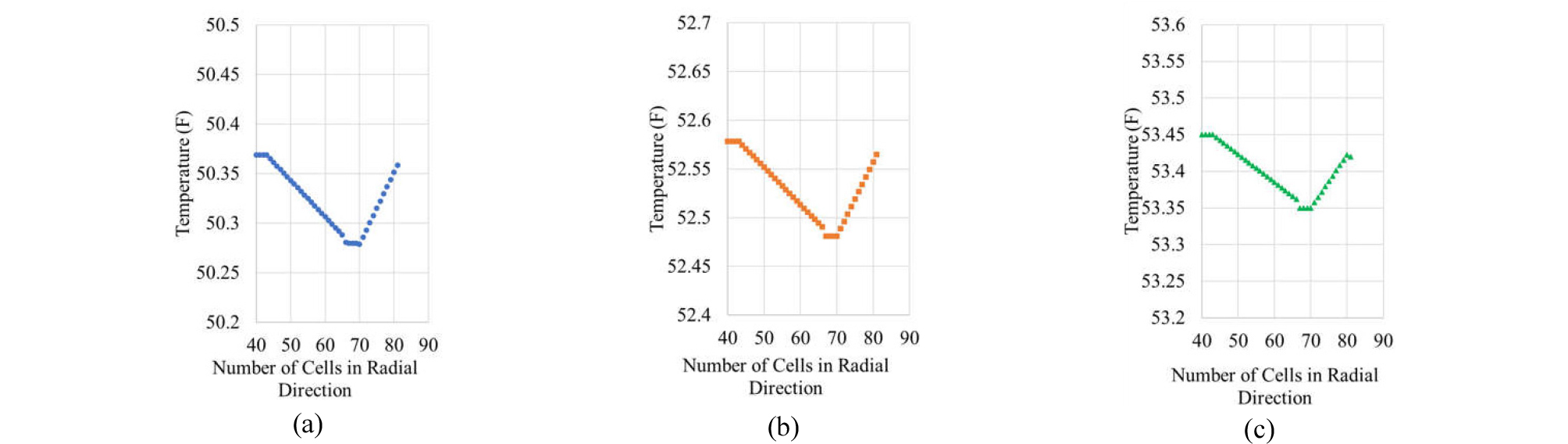
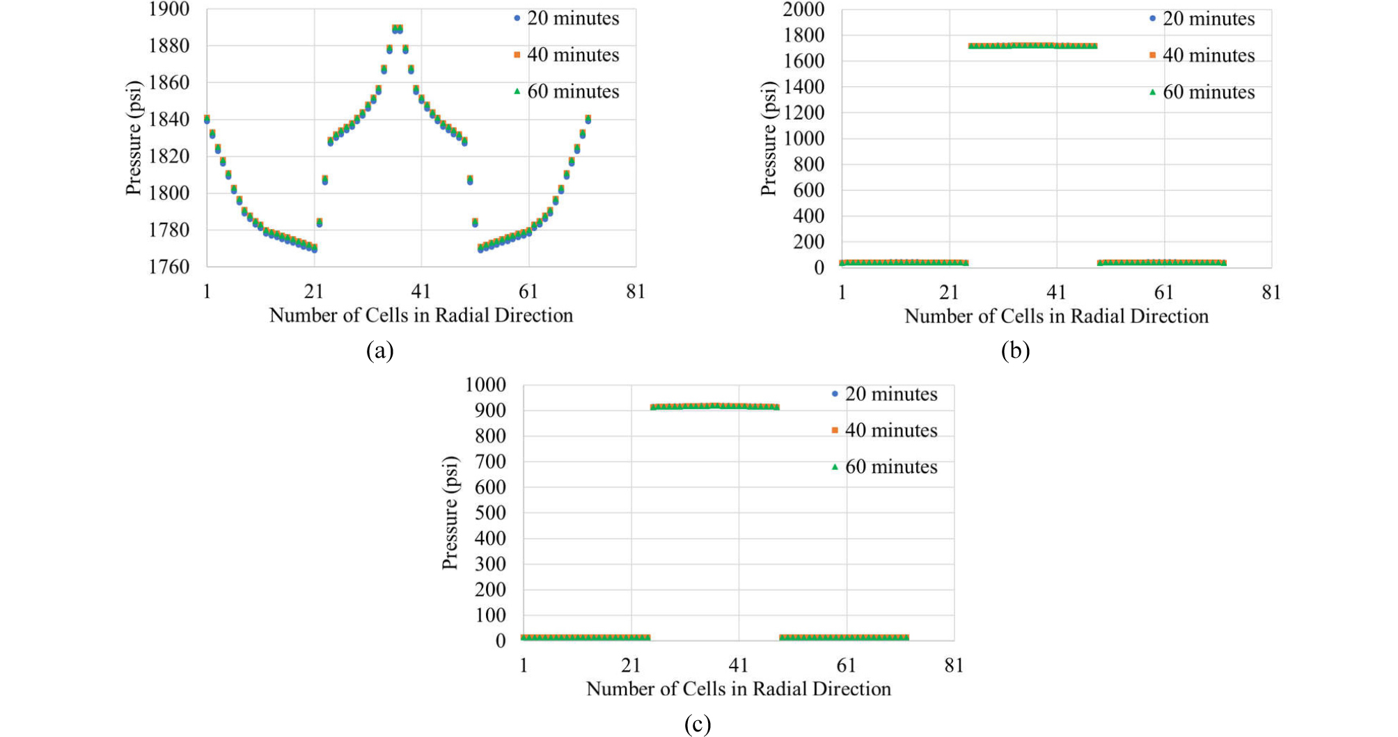
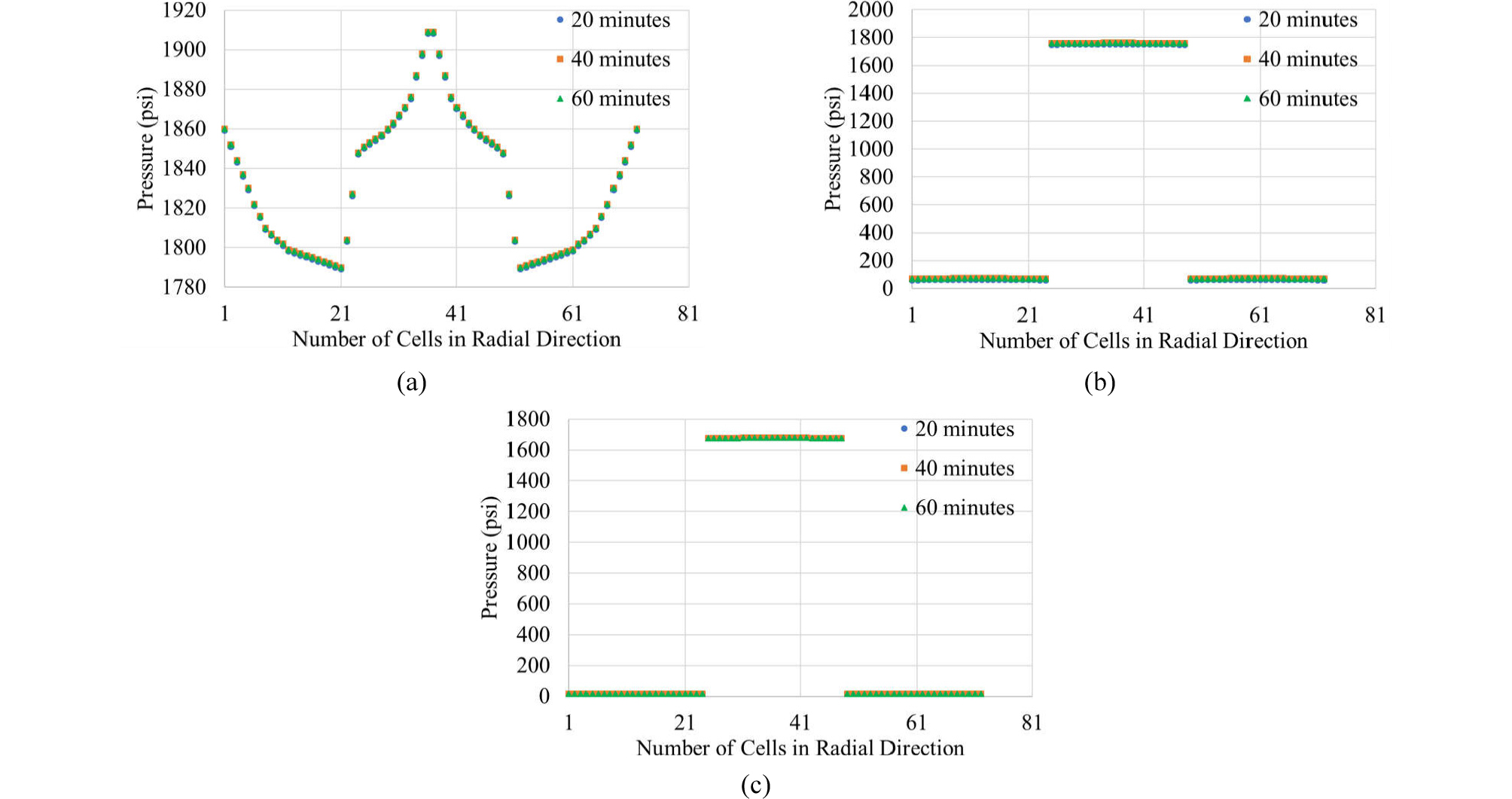
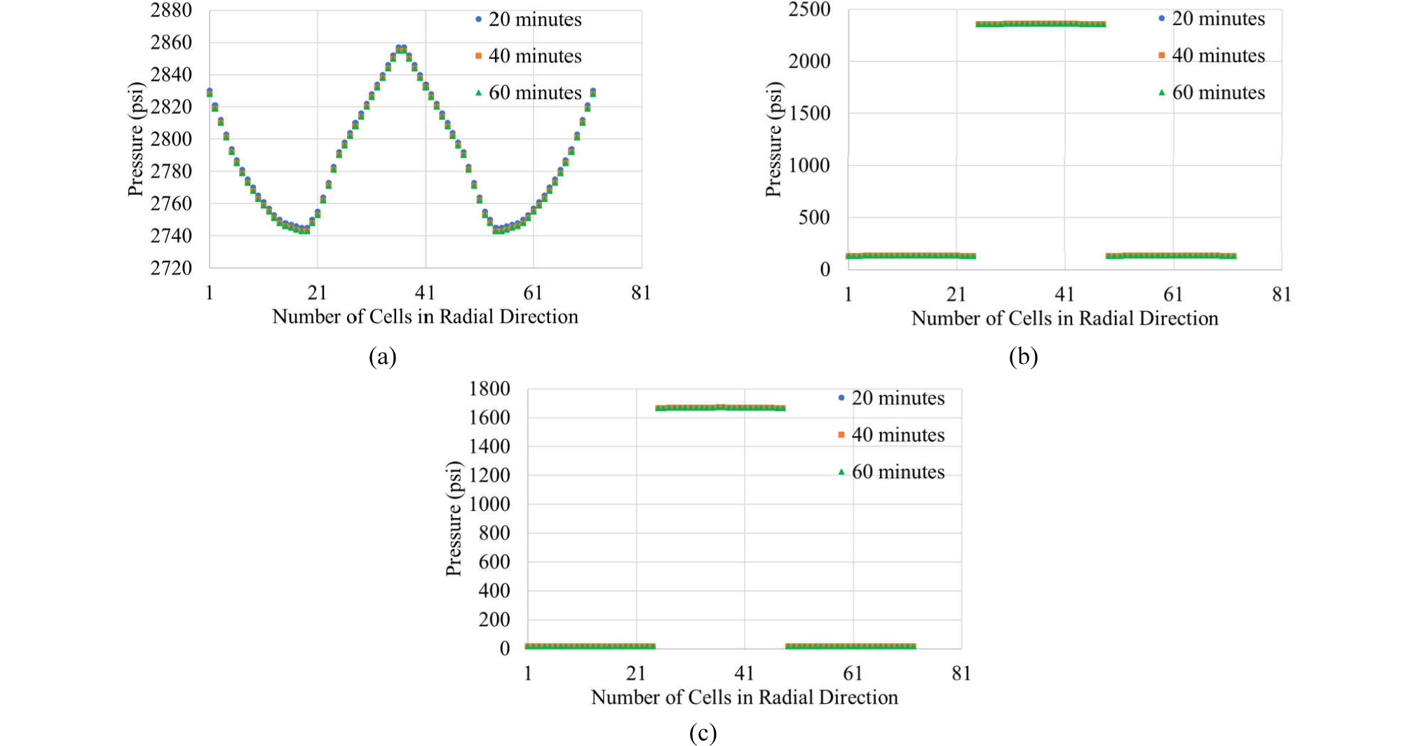
In order to understand the difference between 1D and multi-dimensional simulation further, Fig. 14 shows the distribution of temperature along the radial direction for the full system at z = 5,721 ft for base scenario (i.e., formation - casing - annulus - pipe) at three different times (t = 20, 40, and 60 minutes). Fig. 15 shows the same plots without formation so that the temperature distribution along radial direction within casing - annulus - pipe at t = 20, 40, and 60 minutes could be magnified. As conjectured from Figs. 11 through 13, there are as much as 0.2oF temperature variations both in the pipe and annulus at the same depth. Such variations require more time for heat transfer compared to 1D simulation, which supports the results in Figs.4 through 6. One may see that magnitude of temperature difference (0.2oF) trivial but, when it comes to the time associated, it ranges as much as 10 minutes (see the gentle slopes of the curves in Figs. 4 through 6) that corresponds 1/6 (about 16.7%) of overall operation time.

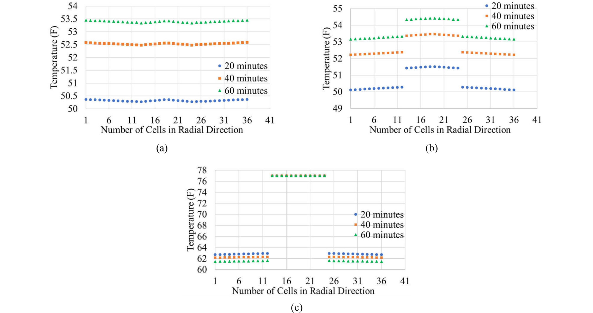
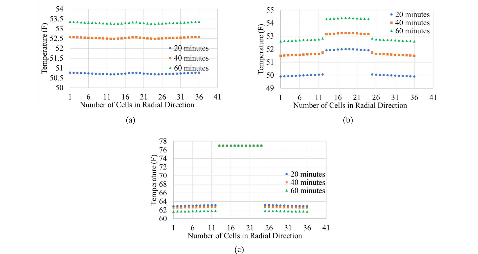
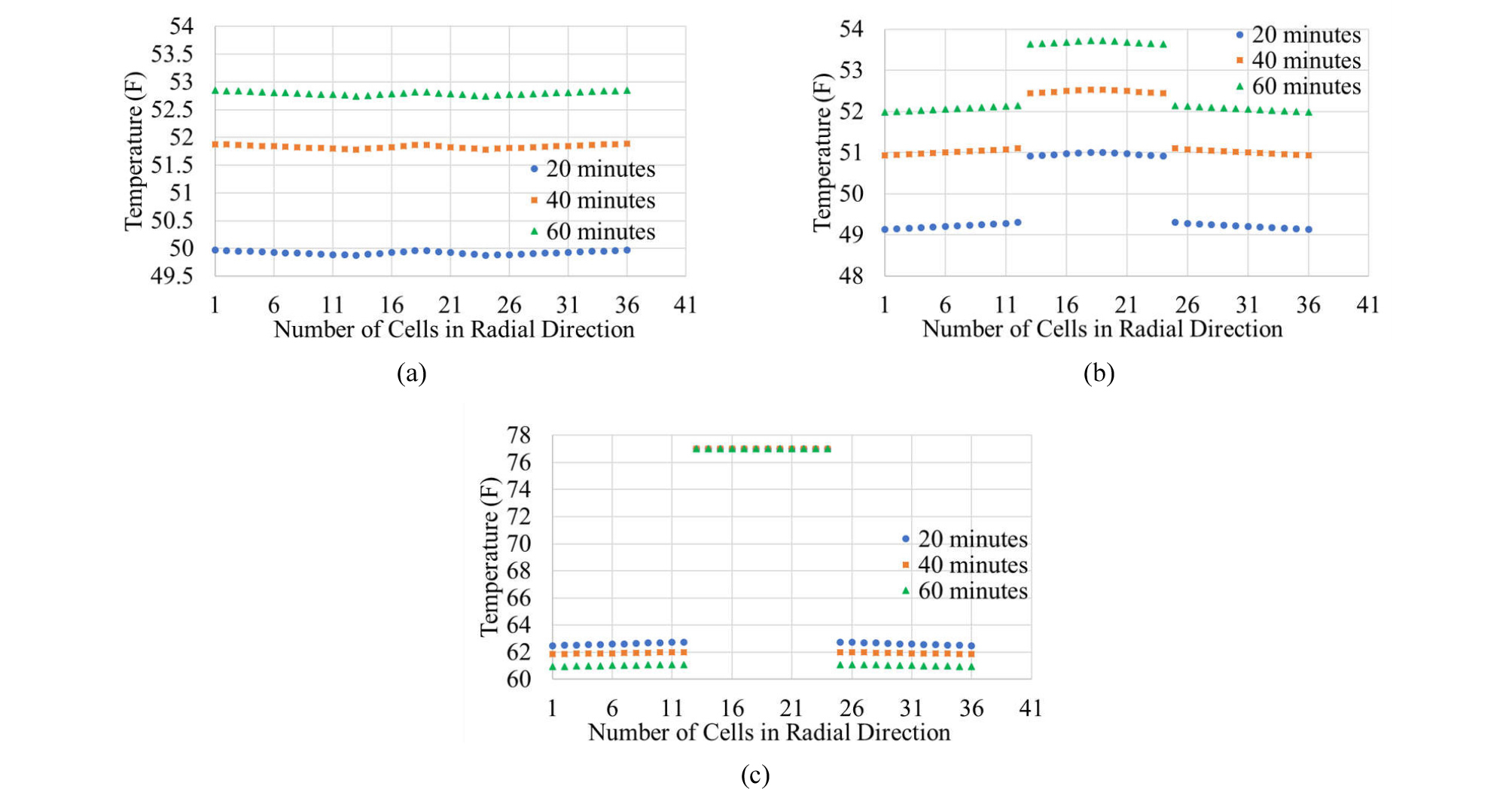
Figs. 16 through 18 show the distribution of temperature along the radial direction within the flowing area (annulus and drill pipe) for base scenario (cf. Figs. 14 and 15), scenario 1, and scenario 2, respectively, at t = 20, 40, and 60 minutes at the three monitoring locations of z =5,721 ft, z = 4,786 ft, and z = 0 ft. In all scenarios (at different locations and times), temperature variations along the radial direction are shown to exist consistently in multi-dimensional simulations.
Such radial variations can also be shown in terms of pressure, as shown in Figs. 19 through 21 that can be paired with Figs. 16 through 18.
Conclusions
This study investigates multi-dimensional simulations of transient temperature profile during fluid circulation to help designing future offshore cementing process by using, ANSYS Fluent. When the simulation results are compared with field tests and one-dimensional (1D) simulation results available in the literature, the following conclusions can be made:
(1) The two-dimensional simulation result in this study, through convection and conduction, predicts similar trends as presented by the field tests and 1D simulation result in the literature. In all three monitoring locations (near the bottom hole, surface, and middle of the well), it predicts a longer time for heat transfer.
(2) A delay in heat transfer is shown to be caused by non-uniform distribution of velocity profile within the drill pipe as well as annulus, which in turn is affected by flow rheology and the way fluids are distributed in the well. Such an effect is pronounced at the bottom hole where the injected fluid is stripping off the existing fluid from the outer edge.
(3) Additional simulations with seawater injection into a well filled with drilling mud (scenario 1) and mud injection into a well filled with seawater (scenario 2), on the top of seawater circulation (base scenario), show that fluid-fluid interactions at the interface can also contribute to heat transfer to some degree.
