General Remarks

Journal of the Korean Society of Mineral and Energy Resources Engineers. 31 October 2020. 506-526
https://doi.org/10.32390/ksmer.2020.57.5.506

ABSTRACT


MAIN

  • 서 론

  • 전기비저항 탐사의 원리 및 측정 시스템

  •   원리

  •   측정시스템

  •   전극배열

  • 탐사 방법

  •   시추공 토모그래피

  •   전기비저항 모니터링

  • 모델링 및 역산

  •   모델링

  •   역산

  • 적용사례

  •   광물자원탐사

  •   지하수 조사

  •   환경오염대 조사

  •   토목물리탐사

  •   유적물리탐사

  •   농업물리탐사

  • 결론 및 전망

서 론

전기비저항 탐사는 다양한 물리탐사법 중 가장 널리 사용되는 물리탐사법 중 하나로, 전통적인 지하광물자원 탐사는 물론 토목, 지하수, 환경, 유물조사 등 다양한 분야에 적용되고 있다. 전기비저항 탐사는 지표 및 시추공에서 널리 적용되고 있으며, 육상은 물론 하상, 해상에서도 활발하게 적용되고 있다. 특히 국내의 경우 대지의 전기비저항이 높아 양질의 자료획득이 가능하다는 점이 전기비저항 탐사의 적용성을 높이는데 크게 기여하였다.

전기비저항 탐사는 1883년 광물탐사에 최초로 적용되었으며, 1913년에는 시추공 탐사에 적용된 바 있다(Rust, 1938). 이후 Wenner(1912, 1915)와 Schlumberger(1920)는 겉보기 전기비저항(apparent resistivity) 개념을 도입하여 전기비저항 탐사 자료의 해석에 전환점을 마련하였으며, Tikhonov(1943)는 전기비저항 영상화 기법을 제시하였다. 이러한 전기비저항 탐사법은 1920년대 초 최초로 현장 탐사가 수행된 이래 1980년대까지 1차원 탐사가 성행하였으며, 이후 2차원 탐사가 도입되었고, 3차원 및 4차원 탐사로 확대 발전되었다. 이러한 획기적 발전은 측정 장비의 정밀도 향상, 자료획득 기술, 해석 이론 및 소프트 웨어의 발달에 기인한다.

이 총설에서는 지난 20년 동안 전기비저항 탐사 분야의 핵심적인 발달을 요약하고자 한다. 우선 간략하게 전기비저항 탐사의 원리를 소개하고, 2~4차원 전기비저항 탐사 현장 자료획득, 자료처리 및 해석과 관련된 최근의 기술개발과 연구동향을 기술하고, 마지막으로 그 적용성과 향후 발전방향을 분석하였다.

전기비저항 탐사의 원리 및 측정 시스템

원리

전기비저항 탐사는 한 쌍의 전류전극을 통하여 직류전류를 지하에 주입하고, 다른 한 쌍의 전위전극에서 전위차를 측정하여 지하의 전기비저항 분포를 영상화하는 방법이다. Fig. 1에 주어진 바와 같이 한 쌍의 전류전극을 통하여 지하에 전류를 주입하면 1차 전위(primary potential)를 만들어 내며, 이 1차장에 의해 배경매질과 전기비저항이 다른 이상체의 표면에 표면전하가 발생한다. 이 표면전하는 2차(secondary) 전기장 및 전위를 생성한다. 전기비저항 탐사는 한 쌍의 전위전극에서 1차장과 2차장의 합인 합성장의 전위차를 측정하여 지하의 전기비저항 분포를 영상화하게 된다. 이때 생성되는 표면전하의 양은 배경매질과 이상체의 전기비저항 차에 비례하며, 그 분포 양상은 전류전극에 의한 1차장과 이상체의 기하학적 특성에 좌우된다.
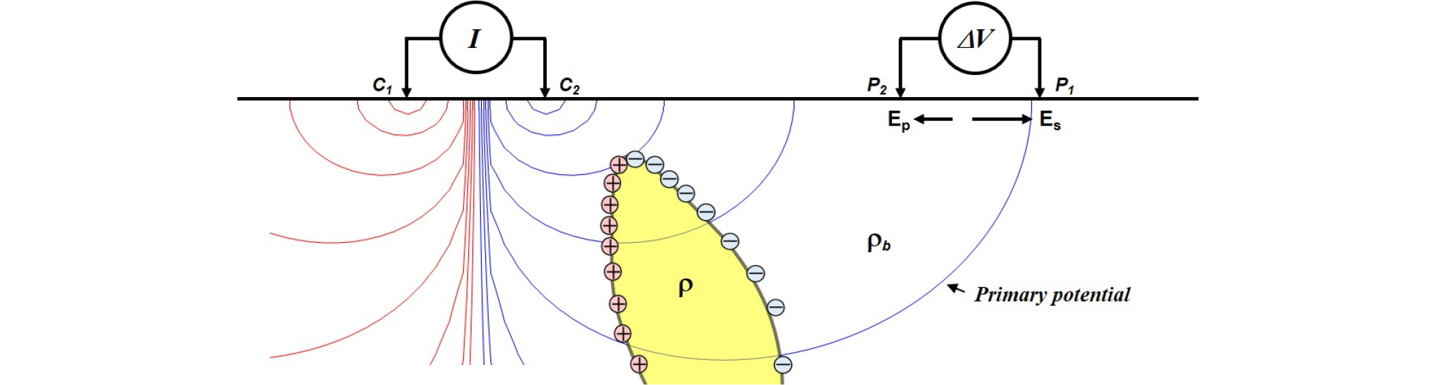
http://static.apub.kr/journalsite/sites/ksmer/2020-057-05/N0330570511/images/ksmer_57_05_11_F1.jpg
Fig. 1.

A conductive model excited by a dipole source. The red and blue lines represent the positive and negative equipotential lines of the primary potential. The surface charges arise to reduce the primary electric field in the conductive body and produce the secondary electric field inside and outside the body.

전기비저항 탐사에서 측정되는 양은 전위전극 사이의 전위차인 반면, 전기비저항 탐사를 통하여 알아내야 하는 양은 전기비저항이다. 또한 전위차는 전류원과 측정점 사이의 거리에 따라 민감하게 변화한다는 문제점을 가지고 있다. 즉 균질 반무한 공간의 경우에도 측정되는 전위차는 측정점의 위치에 따라 달라진다. 이러한 문제를 해결하기 위하여 전기비저항 탐사에서는 측정된 전위차를 다음과 같이 겉보기 전기비저항(apparent resistivity) ρa로 변환하여 해석에 사용한다(Wenner, 1912, 1915).

$$\rho_a=\rho_b\frac{\Delta V}{\Delta V_p}$$ (1)

(1)식에서 ΔVp는 전기비저항 ρb인 균질 반무한 공간에서의 1차 전위차, V는 측정된 전위차를 나타낸다. 겉보기 전기비저항은 매질이 균질한 경우에는 참 전기비저항 값과 같지만, 대개의 경우 참 전기비저항과는 다른 값을 보인다. 따라서 겉보기 전기비저항이 지하의 참 전기비저항을 의미하지는 않지만, 적어도 전기비저항의 단위를 가지며, 가단면도(pseudo-section) 등으로 나타내면 지하의 전반적인 전기비저항 분포를 파악하는 데 도움이 된다.

측정시스템

전기비저항 탐사 자료획득 시스템은 전류전극과 전위전극, 전극과 측정 시스템을 연결하는 케이블, 그리고 측정 시스템으로 구성된다. 전극은 지하에 전류를 주입하거나 전위를 측정하기 위한 송신 및 수신부에 해당하며, 일반적으로 금속봉 전극이 널리 사용된다. 초기에는 비분극 전극(non-polarizable electrode)을 사용하기도 하였으나 비분극 전극은 제작 및 유지관리가 어렵고, 설치가 번거롭기 때문에 현재 거의 사용되지 않는다. 그러나 금속봉 전극의 설치가 어려운 환경에서는 다양한 형태의 전극을 사용할 수 있다. 예를 들어 시멘트 포장된 도로의 경우에는 평판 전극(plate electrode) 등이 사용된다. 전극은 단지 지하매질에 전류를 주입하고, 전위를 측정하는 기능만 수행하면 되며, 이를 위해서는 지하매질과 전극의 접촉이 긴밀히 유지되면 된다. 한편 최근에는 용량결합전극(capacitive electrode)이 개발되어 비접촉식 탐사의 수행도 가능해졌다(Kuras et al., 2006). 그러나 이 방법은 아직까지는 양질의 자료획득이 쉽지 않으며, 가탐심도가 수 m에 지나지 않다는 문제점이 있다.

초기 전기비저항 탐사에서는 전극과 측정기기의 연결에 단선(single core) 케이블이 사용되었다. 따라서 측선상의 여러 측점에서 자료를 획득하는 2차원 이상의 탐사에서는 자료획득에 많은 시간이 소요된다. 1990년대 이후에는 각 측점에 전극을 미리 설치한 다음, 다중(multi-core) 케이블을 사용하여 측정기기와 각각의 전극을 연결하는 방법이 도입되었다. 다중 케이블은 다중채널 자동 측정기기와 함께 최근의 전기비저항 탐사에서 예외 없이 적용되고 있으며, 자료획득의 생산성 향상에 크게 기여하였다. 다중 케이블 도입 초기에는 유도결합(inductive coupling)에 의한 잡음의 문제가 제기되기도 하였으나 실험을 통하여 큰 문제가 없음이 밝혀졌다.

전기비저항 측정 시스템은 앞서 언급한 바와 같이 다중채널(multi-channel), 자동측정 기능이 탑재된 시스템이 주류를 이루고 있다. 상대적으로 단일채널, 수동측정 시스템에 비하여 가격이 높지만, 현장 자료획득에 소요되는 시간과 인력의 절감 효과가 뛰어나 단일채널 수동측정 시스템은 점차 사라지는 추세이다. 또한 보다 양질의 자료획득을 위하여 송신원의 출력도 점차 높아지고 있다. Table 1에 현재 국내에 다수 보급된 상업용 전기비저항 측정 시스템의 사양을 요약하였다.

Table 1.

Commercial resistivity measuring systems

Model Manufacturer Channel Auto. IP Max. Current(mA)
Super Sting R8 AGI 8 y y 2000
Syscal Pro Iris 10 y y 2500
Lund system ABEM 4 y y 1000

전극배열

전기비저항 탐사에서는 다양한 전극배열법이 사용되며, 서로 다른 전극배열은 서로 다른 신호 크기, 가탐심도 및 분해능을 갖는다. 따라서 조사 목적 및 탐사 대상지역의 특성에 따라 적정한 전극배열법을 선정하는 것은 양질의 자료획득은 물론 해석결과의 신뢰도 향상에 크게 기여한다. Fig. 2는 전기비저항 탐사에서 널리 사용되는 전극배열법을 나타나낸 것이며, 이들 전극배열법의 특성에 관한 많은 연구결과가 발표된 바 있다(Oldenburg and Li, 1999; Dahlin and Zhou, 2004; Saydam and Duckworth, 1978; Kim et al., 2001; Zhou et al., 2002; Szalai and Szarka, 2008).

http://static.apub.kr/journalsite/sites/ksmer/2020-057-05/N0330570511/images/ksmer_57_05_11_F2.jpg
Fig. 2.

Typical electrode configurations used in electric resistivity measurement: (a) Wenner, (b) Schlumberger, (c) pole-pole, (d) pole-dipole and (e) dipole-dipole array.

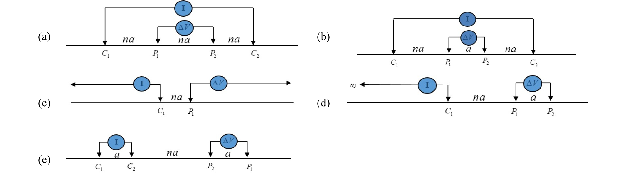
Table 2는 대표적인 전극배열법에 대한 특징을 요약한 것이다(Okpoli, 2013). 단극배열은 분해능은 낮지만 가탐심도가 크다는 장점이 있으며, 슐럼버져 및 웨너 배열은 수직분해능이 높아 수직탐사에, 단극-쌍극자 및 쌍극자 배열은 신호대 잡음비와 가탐심도 측면에서 약점이 있으나, 수평분해능이 높아 2차원 탐사에 널리 사용되고 있다. 이들 고전적인 전극배열법은 각각의 장단점을 가지고 있으며, 이를 보완하기 위하여 Kim et al.(2006)은 변형된 단극-쌍극자 배열 등 다양한 전극배열법을 제시하였다.

Table 2.

Characteristics of typical electrode arrays (Okpoli, 2013). Each star represents the degree of effectiveness of the array (4 stars being most effective)

Wenner Schlumberger Pole-pole Pole-dipole Dipole-dipole
Horizontal resolution * ** ** ** ****
Vertical resolution **** *** ** * ***
Depth of investigation * ** **** *** ***
Signal strength **** *** **** ** *

탐사 방법

전기비저항 탐사는 지하의 구조에 따라 1차원, 2차원 및 3차원 탐사로 구분된다. 또한 최근에는 시간적 변화를 고려하여 4차원 탐사로 그 영역을 확대하고 있다. 한편 조사 위치에 따라 지표탐사, 시추공 탐사, 수상 탐사로 분류할 수 있다. 여기서는 지표탐사를 기준으로 1차원에서 3차원 탐사 방법을 기술하고, 토모그래피 탐사 및 모니터링 조사를 기술한다.

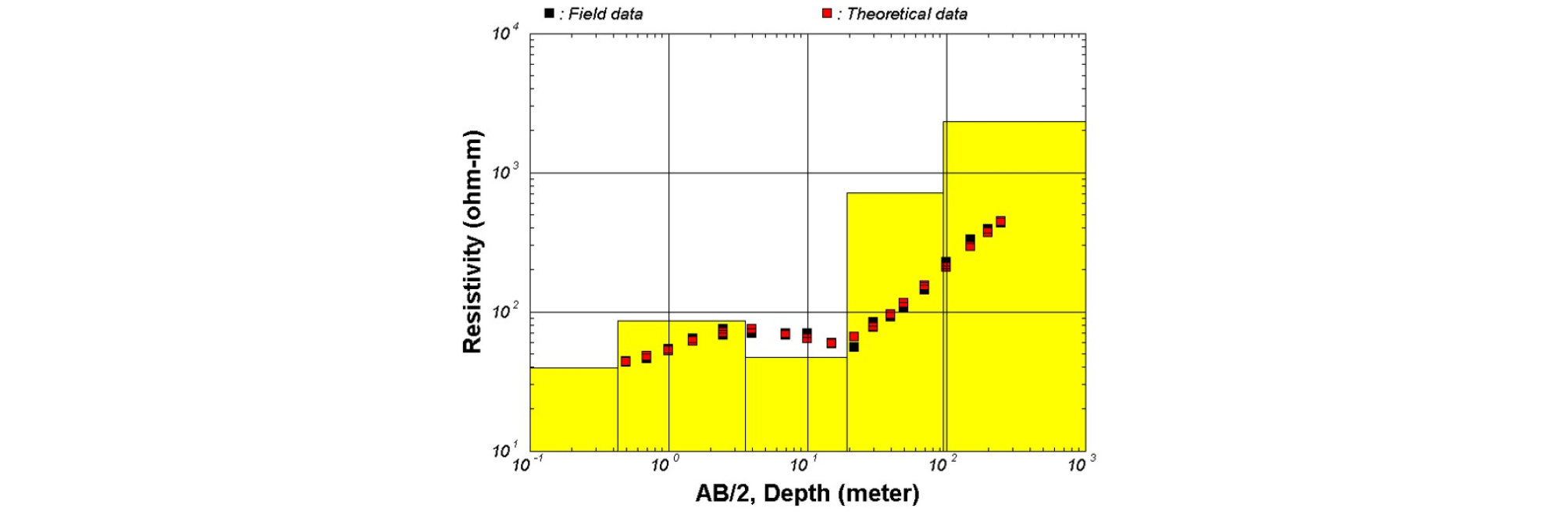
지하가 1차원, 즉 수평다층 구조일 경우에는 전기비저항은 수평방향으로 변화가 없고, 수직방향으로만 변화한다. 따라서 전기비저항 탐사에서는 수직방향으로의 전기비저항 변화를 파악해야 하며, 이러한 목적으로 수행되는 전기비저항 탐사는 1차원 탐사 혹은 전기비저항 수직탐사(sounding)라 불린다. 전기비저항 수직탐사에서는 측정점을 중심으로 전류전극 간격을 넓혀가면서 자료를 획득하며, 전류전극 간격이 좁은 자료는 천부, 넓은 자료는 심부의 정보를 제공한다. 따라서 전기비저항 1차원 탐사는 기하학적 수직탐사(geometric sounding)에 해당한다. 1차원 탐사의 목적은 전기비저항의 수직 방향 변화를 알아내는 것이다. 따라서 수직탐사에서는 수직분해능이 뛰어난 슐럼버져나 웨너배열이 사용된다. 전류전극을 증가시키면서 측정된 자료는 Fig. 3에 나타낸 것처럼 수직탐사 곡선(sounding curve)을 작성하고, 이를 역산하여 각 층의 두께 및 전기비저항을 추정한다. 그러나 1차원 탐사는 전기비저항을 수평적 변화를 고려하지 못한다는 결정적 단점을 가지고 있어, 특별히 층서구조를 보이지 않는 지역에 적용하기에는 한계가 있다.

http://static.apub.kr/journalsite/sites/ksmer/2020-057-05/N0330570511/images/ksmer_57_05_11_F3.jpg
Fig. 3.

Example of a resistivity sounding curve and its inverted 1D model.

2차원 탐사는 지하의 물성(전기비저항)이 주향방향으로 변화가 없다고 가정하고, 직선형의 측선상에서 수평탐사 및 수직탐사를 동시에 수행하는 방법이다. 2차원 탐사는 측선하부의 수평 및 수직방향의 전기비저항 분포를 영상화할 수 있다. 2차원 탐사에서 얻어진 자료는 소위 겉보기 전기비저항 가단면도 형태로 기록된다. 2차원 탐사에서는 주로 수평 분해능이 뛰어난 단극, 단극-쌍극자 및 쌍극자 배열이 적용되며, 대지의 전기비저항이 높아 신호의 크기가 큰 국내의 경우에는 수평 분해능이 가장 뛰어난 쌍극자 배열을 선호한다. 그러나 전기비저항이 낮은 지역, 예를 들어 석탄층 지역, 해안지역, 폐기물 오염지역 등에서는 신호가 작을 수 있으므로 단극 배열과 같이 신호가 큰 배열을 사용하는 것이 효과적이다. 최근에는 다중채널, 자동측정 시스템이 도입되면서 다양한 배열의 자료를 모두 얻어 해석에 사용하는 방법도 사용된다. 2차원 탐사자료의 해석은 일반적으로 역산을 통하여 측선하부의 전기비저항 분포를 영상화하는 기법이 사용된다. 전기비저항 2차원 역산 소프트웨어에는 Dipro, GeoTomo(Loke, 2012) 등이 있으며, 국내의 경우에는 대개 Dipro가 사용되고 있다. 이들 소프트 웨어는 자료처리 및 해석에 이르는 전 과정이 자동화되어 있으며, 개인용 컴퓨터에서 매우 빠르게 수행된다.

Fig. 4는 한국광물자원공사에서 열수광산 광화대 조사를 위하여 수행된 2차원 전기비저항 탐사에서 얻어진 겉보기 전기비저항 가단면도 및 그 역산 결과를 나타낸 것이다 (KORES, 2013). 측점 간격은 20 m 이며, 측선의 총 길이는 460 m이다. 수평방향 130 m 지점 하부에 단층대로 해석되는 낮은 전기비저항 이상대가 나타나고 있으며, 이 단층대를 따라 열수광상의 발달 가능성이 높은 것으로 해석되었다.

http://static.apub.kr/journalsite/sites/ksmer/2020-057-05/N0330570511/images/ksmer_57_05_11_F4.jpg
Fig. 4.

Example of a 2D resistivity survey: (a) apparent resistivity pseudo-section and (b) inverted model.

2차원 전기비저항 탐사는 현재 가장 널리 사용되는 효과적인 지하 영상화기법이지만, 근본적으로 지질 및 지형이 주향방향으로 변화하지 않아야 한다는 조건을 만족해야 한다. 따라서 측선을 가능하면 주향방향에 수직하게 설정해야만 3차원적 변화에 의한 영향을 최소화 할 수 있다. 이러한 문제점에도 불구하고 2차원 전기비저항 탐사법은 현장 자료획득이 용이하고 경제성이 높기 때문에 가장 널리 적용되고 있다.

일반적으로 지하 구조 및 지형을 1차원, 2차원으로 가정하는 데는 한계가 있다. 특히 국내에서와 같이 지질구조가 복잡하고, 지형의 변화가 심한 환경에서 1차원이나 2차원 모델을 가정하는 것은 쉽지 않다. 3차원 탐사는 지하구조 및 지형에 아무런 제한이 없이 지하물성이 3차원적으로 변한다고 가정하므로 가장 정확하게 지하의 3차원 전기비저항 분포를 파악할 수 있는 정밀 탐사법이다. 그러나 3차원 영상화를 위해서는 기본적으로 3차원 해석을 위한 자료가 확보되어야 하며, 자료획득 및 처리에 소요되는 비용이 증가한다. 3차원 탐사에서는 격자망(grid)으로 측점을 설정하고 자료를 획득해야 한다(Park and Van, 1991; Li and Oldenburg, 1992). 그러나 이 경우 자료획득에 너무 많은 시간이 소요되므로, 실제 현장 탐사에서는 조사영역 내에 평행한 여러 개의 종 측선과 횡 측선을 설정한 다음, 각 측선에서 2차원 자료를 획득하는 방법(Rucker et al., 2009a)을 사용한다. 이러한 자료획득 방법은 3차원 탐사의 비용 절감에 매우 효과적이다.

3차원 탐사에는 단극배열이 널리 사용된다. 그러나 이 경우에도 2차원 탐사에서와 마찬가지로 조사목적이나 조사지역의 특성에 따라 최적의 전극배열법을 선택할 수 있으며, 다양한 전극배열에 대한 자료를 동시에 획득할 수도 있다. 3차원 탐사자료의 해석도 역산을 통하여 이루어지며, 비록 계산시간이 길지만 개인용 컴퓨터에서도 충분히 가능하다. 3차원 탐사는 비록 비용이 많이 든다는 단점이 있으나, 복잡한 지질구조를 가장 정확하게 영상화할 수 있은 효과적인 탐사법으로 점차 그 적용이 확대되어 가고 있다.

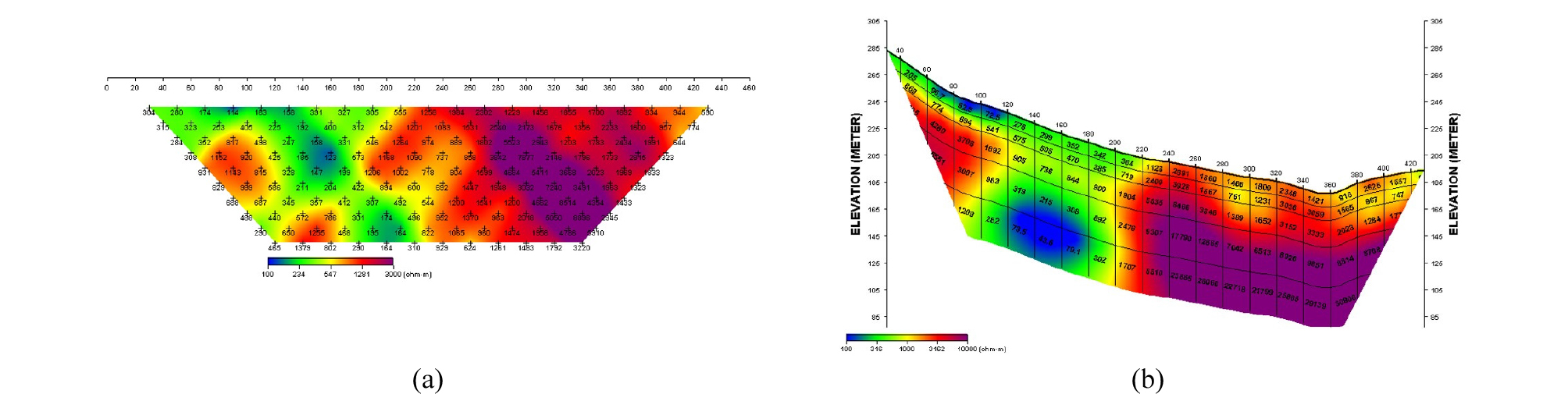
Fig. 5는 저수지 안전진단을 위하여 제체에서 수행된 3차원 전기비저항 탐사 사례를 나타낸 것이다(Cho and Yong, 2019). 측점간격은 5 m 이며, 제체에 평행한 방향 8개 측선(H1~H8)과, 수직한 방향 9개 측선(V1~V9)에서 2차원 탐사를 수행하고, 이들 자료를 병합하여 3차원 역산을 수행하였다. 저수지 제체의 전기비저항 구조를 파악할 수 있으며, 조사용 시추공(S1~S6) 주변에 저비저항 이상대가 발달한 것을 확인할 수 있다.
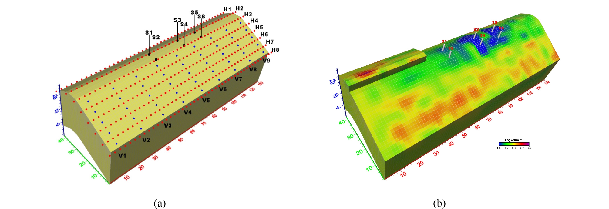
http://static.apub.kr/journalsite/sites/ksmer/2020-057-05/N0330570511/images/ksmer_57_05_11_F5.jpg
Fig. 5.

Example of a 3D resistivity survey at an embankment dam: (a) survey lines and (b) reconstructed 3D resistivity model (after Cho and Yong, 2019).

시추공 토모그래피

지표 전기비저항 탐사는 투사각, 가탐심도 및 분해능의 한계로 인하여 심부의 정밀 영상화가 쉽지 않다. 이의 극복을 위하여 시추공내에서 자료를 획득하는 시추공 전기비저항 토모그래피 탐사가 도입되었다. 전기비저항 토모그래피법은 탄성파 토모그래피와 함께 국내외에서 가장 널리 적용되고 있는 지하 영상화 기법으로 지표 전기비저항 탐사법에 비하여 분해능이 높기 때문에 정밀탐사를 목적으로 사용되며, 연약대 분포 조사, 지반침하 조사, 공동조사, 환경오염대 조사 등에 광범위하게 적용되고 있다.

시추공내에 전극을 설치하는 전기비저항 토모그래피 탐사에서 전극은 전기적으로 긴밀하게 공벽에 접지되어야 한다. 시추공이 나공 상태이고 공내수로 채워진 경우에는 대개 다중 전선에 전극을 연결하는 방식(suspended electrode)이 사용되며, 이 경우 전극의 접지문제는 발생하지 않는다. 반면 시추공 상부에 프라스틱 케이싱이 설치된 구간에서는 케이싱 외부에 링 형태의 전극(ring electrode)을 설치하여 자료를 측정한다(Wilkinson et al., 2006a; Tsokas et al., 2011). 이때 케이싱과 공벽 사이는 모암과 비슷한 전기비저항을 갖는 토사로 충전하여 전극을 공벽에 밀착해야 한다(Wilkinson et al., 2010b).

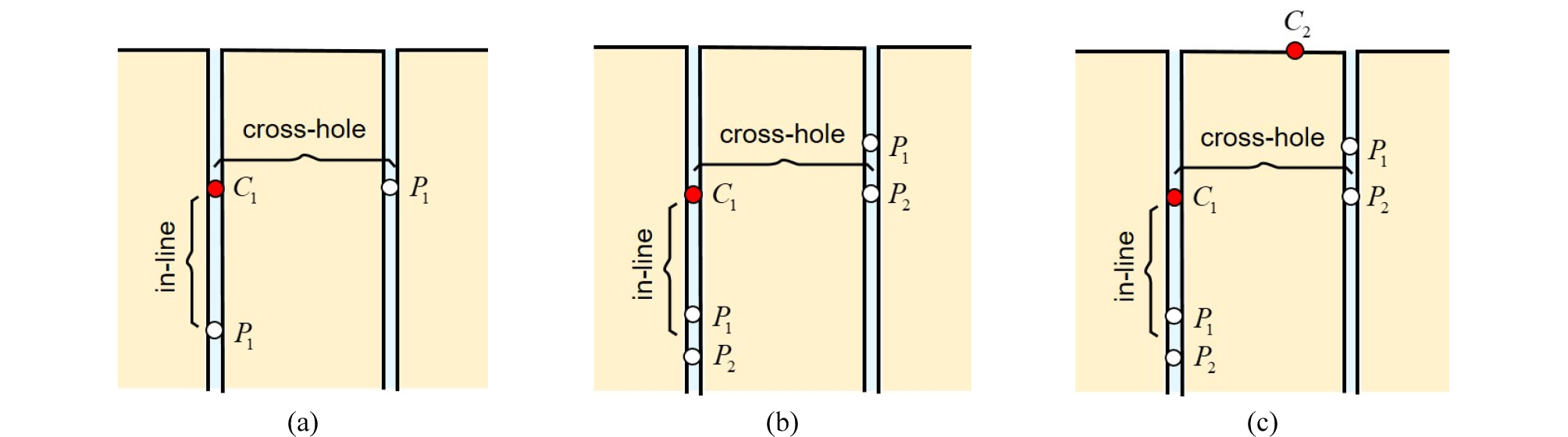
Fig. 6에 나타낸 바와 같이 시추공간 전기비저항 토모그래피 탐사 자료는 크게 시추공-시추공(cross-hole), 동일 시추공(in-line) 및 시추공-지표(hole-to-surface) 자료로 구분된다. 시추공 토모그래피 탐사의 자료획득은 전류전극을 고정시키고 전위전극을 이동시키면서 스캐닝하는 방식을 사용한다. 따라서 통상적인 지표 전기비저항 탐사에 비하여 측정 자료의 수가 많으므로 자동측정이 가능한 측정 장비를 사용하는 것이 바람직하다.

http://static.apub.kr/journalsite/sites/ksmer/2020-057-05/N0330570511/images/ksmer_57_05_11_F6.jpg
Fig. 6.

Data acquisition of resistivity tomography and typical electrode configurations: (a) pole-pole, (b) pole-dipole and (c) modified pole-dipole.

지표탐사에서와 마찬가지로 시추공 토모그래피 탐사에서도 다양한 전극배열법을 사용할 수 있으며, 각 배열법은 서로 다른 분해능과 가탐반경을 가진다. 그러나 지표탐사와는 달리 서로 다른 시추공에 전류 및 전위전극이 위치하는 시추공-시추공 자료에서는 1차 전위차(Vp)가 0이 되어 겉보기 전기비저항이 발산하는 무결합(null coupling) 영역이 존재한다(Cho et al., 1997a; Nimmer et al., 2008; Lee et al., 2016a). 이 경우 (1)식에 주어진 겉보기 전기비저항이 발산하므로 자료 역산에 문제가 발생한다. 무결합 문제가 발생하는 영역은 전류전극과 전위전극의 기하학적 위치에 의해 결정되며, 단극-쌍극자 배열, 쌍극자 배열에서 뚜렷하다. Kim et al.(2006)은 이러한 문제점의 해결을 위하여 변형된 단극-쌍극자 배열을 제안하였으며, 이 배열은 단극-쌍극자 배열과 유사한 분해능을 유지하면서도 무결합 영역을 현저히 줄여주는 효과가 있다. 또한 전기비저항 토모그래피 탐사에서 동일 시추공 자료는 결과영상의 분해능을 크게 향상시키므로 필수적으로 측정되어야 한다. 그러나 시추공이 모암에 비하여 전기비저항이 매우 낮은 공내수로 채워진 경우, 동일 시추공 자료, 특히 전류전극과 전위전극이 가까운 경우에는 소위 공내수 효과(borehole effect)에 의해 동일 시추공 자료는 크게 왜곡된다(Cho et al., 1997b; Osiensky et al., 2004; Nimmer et al., 2008). Lee et al.(2016a)은 공내수 효과를 포함한 역산을 통하여 보다 참 모델에 근접한 역산 영상을 추정함을 확인하였다.

전기비저항 토모그래피에 관한 연구는 1980년대 중반에 출발하여 2차원 전기비저항 토모그래피(Shima and Sakayama, 1987; Dailly and Owen, 1991; Sasaki, 1992; Daily and Ramirez, 1995; LaBrecque et al., 1996; Zhou and Greenhalgh, 2000; Deceuster et al., 2006; Tsourlos et al., 2011), 3차원 전기비저항 토모그래피(Shima, 1992; Wilkinson et al., 2006b; Yi et al., 2006; Nimmer et al., 2008), 최적 탐사 설계(Wilkinson et al., 2012), 시추공내 전극의 위치 오차(Oldenborger et al., 2005; Wilkinson et al., 2008)와 시추공 편향(Yi et al., 2009), 전기비저항 이방성(Kim et al., 2006; Yi et al., 2011)에 관한 연구가 수행되었다.

전기비저항 모니터링

통상적인 전기비저항 탐사에서 지하의 전기비저항 구조는 시간에 따라 변화하지 않는다고 가정한다. 그러나 경우에 따라서는 지하의 시간적 전기비저항 변화대 탐지가 주된 탐사 목적이 될 수 있다. 전기비저항 모니터링은 일정 시간 간격으로 자료를 수집하여 지하의 시간에 따른 전기비저항 변화대를 파악하는 탐사 방법이다. 이러한 전기비저항 모니터링은 자동 측정 기술과 통신 기술 및 해석기술의 발달에 힘입어 급속히 발전하고 있으며, 지하수(Park, 1998; Slater et al. 2000; Day-Lewis et al., 2002; Cassiani et al., 2006; Oldenborger et al., 2007; Tsourlos et al., 2008; Kim et al., 2009; Coscia et al., 2012), 환경(Daily et al., 1992; Supper et al., 1997; Yaramanci, 2000; Rucker et al., 2011; Park et al., 2016b), 댐 안전진단 및 지반조사(Kim et al., 2007; Yi et al., 2005; Park et al., 2002; Sjödahl et al., 2008), 지질재해(Supper et al., 2008, 2009; Wilkinson et al., 2010a; Kim et al., 2013), 자원개발(Rucker et al., 2013) 등 다양한 분야에 빠르게 확대 적용되고 있다.

현재 전기비저항 모니터링 시스템은 다중채널 및 자동측정 기능이 탑재되어 있어 일정 시간 간격으로 자료를 수집하고, 인터넷 기반 통신망을 통하여 본부에 설치된 저장 장치(data base)에 자동 저장된다. 또한 양방향 통신을 통하여 모니터링 자료획득 변수의 조정이 가능하다. 전기비저항 모니터링은 지하에 발생하는 전기비저항의 미세한 시간적 변화대도 탐지 가능해야 하므로, 일반적인 일회성 전기비저항 탐사에 비하여 더 정밀한 자료가 요구된다. 또한 가능하면 동일한 탐사변수(전극위치, 전극배열 등)를 적용하여 일정 시간마다 자료를 수집해야 효과적인 해석이 가능하다. 이러한 이유로 전기비저항 모니터링에서는 전극을 영구 매설하는 방식을 선호한다. 전기비저항 모니터링에는 대개 2차원 탐사가 적용되고 있으며, 필요에 따라서는 3차원 탐사 및 시추공 토모그래피 모니터링이 수행되기도 한다(Han, 2019).

전기비저항 모니터링 자료의 해석에는 시간경과 역산법(time-lapse inversion)이 사용된다. 전기비저항 모니터링 초기에는 기준자료와 시간경과 자료를 독립역산(independent inversion)하고, 그 역산영상을 상호 비교하는 방법이 사용되었다(Cassiani et al., 2006). 그러나 이 방법은 미세한 지하의 시간적 변화대 탐지가 어려우며, 각종 역산잡음에 의해 해석결과가 왜곡될 수 있다. 이러한 문제점의 해결을 위하여 시간경과 자료의 역산에 교차 모델제한자(cross-model constraint)를 도입하는 방법이 개발되었으며, 최근에는 모든 모니터링 자료를 동시에 역산하여 지하의 시·공간적 변화를 영상화할 수 있는 4차원 역산(4D inversion)으로 발전하였다.

그러나 전기비저항 모니터링은 아직도 자료획득, 처리 및 그 해석에 있어 개선해야 할 다양한 문제점이 남아있다. 우선 자료수집에서 영구 매설 전극의 부식, 측정기기와 전극을 연결하는 전선의 내구성, 낙뢰에 의한 시스템 망실 등의 문제는 시급히 해결되어야 한다. 또한 모니터링은 일정 시간 간격마다 측정이 이루어지므로 측정된 자료의 양이 방대하다. 따라서 방대한 모니터링 자료의 처리 및 해석을 위해서는 모든 과정이 자동화되고 신속해야 한다. 특히 모니터링에서 축적된 시계열(time-series) 자료에는 다양한 형태의 잡음이 존재하며, 이들 잡음은 자료처리 과정에서 효과적으로 제거되어야 한다. 효과적인 잡음제거를 위한 필터링 기법, 적정 시간대역(time window)의 설정, 샘플링 간격의 조정, 자료 결손 구간의 처리 등 역산 해석 이전에 선처리(pre-processing) 기법에 대한 체계적인 연구가 요구된다. 또한 4차원 역산도 아직 해결해야 할 다양한 문제점이 남아 있다. 특히 미세한 시간적 변화대를 정밀하고 선명하게 영상화하기 위한 시·공간 모델제한자의 최적화는 4차원 역산의 중요한 연구과제 중의 하나이며, 시간경과에 따른 물성 변화대를 효과적으로 영상화하기 위한 다양한 모델제한자의 개발이나 새로운 역산 알고리듬의 개발도 필요하다.

모델링 및 역산

전기비저항 탐사 자료의 해석은 측정된 겉보기 전기비저항 자료를 역산하여 지하의 참 전기비저항 모델을 영상화하는 방법을 사용한다. 역산에는 많은 방법이 있으나 주로 반복적 최소제곱법이 널리 사용된다. 이 방법은 현장에서 측정한 자료와 추정된 모델에 대한 이론자료 사이의 오차가 최소가 되는 지하 모델을 반복적 방식에 의해 추정하는 역산법다. 따라서 역산에서는 정확한 모델링이 요구되며, 역산의 안정성을 확보하기 위하여 적정한 모델제한을 가해야 한다. 여기서는 탐사자료의 해석을 위한 전기비저항 탐사 모델링 및 역산에 대하여 기술한다.

모델링

전기비저항 탐사 모델링은 지하의 전기비저항 분포로부터 전류원에 의한 전위차와 겉보기 전기비저항을 계산하는 과정이다. 점 전류원(point source)에서 r만큼 떨어진 점에서의 전위는 ohm의 법칙과 전하량 보존의 법칙을 사용하여 다음과 같이 주어진다.

$$\nabla\cdot(\sigma(r)\nabla\phi(r))=I\delta(r-r_s)$$ (2)

(2)식에서 σ는 전기전도도, ϕ는 전위, I 는 주입전류, rs는전류전극의 위치를 나타낸다.

지하 매질이 수평 다층 구조일 경우, 즉 1차원 모델일 경우에는 (2)식은 해석해(analytic solution)가 존재한다. 지하를 N개의 수평 다층 구조로 가정하면, 점 전류원에서 거리 r인 점에서의 전위는 다음과 같이 간단한 Hankel 적분식으로 계산된다.

$$V(r)=\frac1{2\pi}\int_0^\infty T_1(\lambda)J_0(\lambda r)d\lambda\;\mathrm{with}\;T_i=\frac{T_{i+1}+\rho_i\tanh(\lambda t_i)}{1+T_{i+1}\tanh(\lambda t_i)/\rho_i}\mathrm{and}\;T_N=\rho_N$$ (3)

(3)식의 Hankel 변환은 선형 필터링(Gosh, 1971)에 의해 계산할 수 있으며, 여기서 ρitii번째 층의 전기비저항과 두께, J0는 Bessel 함수이다.

2차원 및 3차원 모델링은 특별한 경우를 제외하면 해석해가 존재하지 않으므로, 유한차분법(Dey and Morrison, 1979a,b; Spitzer, 1995; Zang, et al., 1995; Loke and Barker, 1996a,b), 유한요소법(Coggon, 1971; Holcombe and Jiracek, 1984; Queralt et al., 1991; Li and Spitzer, 2002) 및 적분방정식법(Hohmann, 1975; Beasely and Ward, 1986) 등 수치적 방법을 사용해야 한다. 적분방정식법은 정확성이 뛰어나고, 이상체만을 분할하므로 단순 형태의 이상체에 대한 모델링에 효과적이지만, 역산으로의 확장성에 제약이 따른다. 이러한 문제점 때문에 2차원 이상의 전기비저항 탐사 모델링에는 미분방정식법인 유한차분법이나 유한요소법이 널리 사용된다. 특이 이들 중에서도 지형의 굴곡 모사가 용이한 유한요소법이 주로 사용된다(Sasaki, 1994; Yi et al., 2001; Rucker et al., 2006).

여기서는 가장 널리 사용되는 유한요소법에 의한 전기비저항 탐사 2차원 및 3차원 모델링에 관하여 기술한다. 2차원 모델의 경우에는 주향방향으로 전기비저항 변화가 없다고 가정하므로 푸리에 변환을 통하여 파수영역(wavenumber domain)에서의 전위 V¯를 계산한다.

$$\overline V(x,\;k_y,\;z)=\int_0^\infty V(x,\;y,\;z)\cos(k_yy)dy$$ (4)

(4)식을 (2)식의 지배방정식에 적용하면

$$\nabla\cdot\left[\sigma(x,\;z)\nabla\overline V(x,\;k_y,\;z)\right]-k_y^2\sigma(x,\;z)\overline V(x,\;k_y,\;z)=-\frac12\delta(x-x_s)\delta(z-z_s)$$ (5)

유한요소법을 사용하여 (5)식의 해를 구하기 위해서는 우선 지하를 작은 크기의 삼각형 혹은 사각형 요소로 분할하고, Galerkin 법을 적용하면 각 절점에서에의 파수영역 전위는 다음의 선형방정식으로 표현된다.

$$\begin{array}{l}\mathbf C\overline{\mathbf V}\boldsymbol=\mathbf s,\\C_{ij}=\int_\Omega\nabla N_i\cdot\nabla N_jd\Omega+k_y^2\int_\Omega\sigma N_iN_jd\Omega+\int_\Gamma\sigma\alpha N_iN_jd\Gamma,\;s_i=\frac12\delta(x-x_s)\delta(z-z_s)\\\alpha=\frac{k_yK_l(k_y\cdot r)\cos\theta}{K_0(k_y\cdot r)} \end{array}$$ (6)

(6)식에서 Ω는 모델링 대상 영역, Γ는 경계 영역, s는 신호원 벡터, N은 각 절점에서의 형상함수(shape function), r은 신호원으로부터 경계요소까지의 거리, θ는 경계면에 수직한 직선과 신호원-경계면을 연결하는 직선이 이루는 각도, K0, K1은 제2종 Bessel 함수이다. (6)식에서 시스템 행렬 C는 대칭 띠 행렬(banded symmetric matrix)이므로 안정적으로 해를 구할 수 있다. 2차원 모델링에서는 여러 개의 파수에 대한 전위를 계산하고, 이를 역푸리에 변환하여 공간영역에서의 전위를 계산한다.

$$V(x,\;y,\;z)=\frac2\pi\int_0^\infty V(x,\;k_y,\;z)\cos(k_yy)dk_y$$ (7)

3차원 모델링의 경우에는 (2)식의 지배방정식은

$$\nabla\cdot\lbrack\sigma(x,\;y,\;z)\nabla V(x,\;y,\;z)\rbrack=-\frac12\delta(x-x_s)(x-x_s)\delta(z-z_s)$$ (8)

로 주어진다. 지하매질을 작은 크기의 사면체 혹은 육면체로 요소분할하고, Galerkin 법을 적용하면 2차원에서 마찬가지로 각 절점에서에의 전위는 다음의 선형방정식으로 표현된다.

$$\begin{array}{l}\boldsymbol C\boldsymbol V\boldsymbol=\boldsymbol s,\\C_{ij}=\int_\Omega\nabla N_i\cdot\nabla N_jd\Omega+\int_\Omega\sigma N_iN_jd\Omega+\int_\Gamma\sigma\alpha N_iN_jd\Gamma,\;s_i=I\delta(x-x_s)(y-y_s)\delta(z-z_s),\\\alpha=\frac{\cos\theta}r. \end{array}$$ (9)

전기비저항 탐사 모델링은 각 측점에서 계산된 전위로부터 (1)식을 사용하여 최종적으로 겉보기 전기비저항 값을 계산한다.

역산

전기비저항 탐사자료의 정량적 해석을 위해서는 반복적 감쇠 최소제곱법(iterative damped least-squares method)이 널리 사용되며, 이는 다음의 목적함수

$$s=\mathbf{\Arrowvert W_d(d-f)\Arrowvert}^{\mathbf2}\boldsymbol+\mathbf{\Arrowvert W_m\triangle P\Arrowvert}^{\mathbf2}$$ (10)

를 최소화하는 모델 증분벡터 Δp를 추정하는 방법이다. (10)식에서 d는 측정자료, 는 주어진 모델에 대한 이론자료이며, Wd는 자료 가중행렬, W은 모델제한자이다. (10)식을 Δp에 대하여 미분하여 0으로 하면, 목적함수를 최소화하는 Δp 다음과 같이 계산된다.

$$\triangle\mathbf p={(\mathbf J^T\mathbf W_d^T{\mathbf W}_d\mathbf J+\mathbf W_m^T{\mathbf W}_m)}^{-1}\mathbf J^T\mathbf W_d^T\mathbf e$$ (11)

여기서 J=f/p로 주어지는 Jacobian 행렬, e=d-f는 측정자료와 모델링에서 계산된 이론자료 사이의 오차를 나타낸다.

전기비저항 탐사자료의 역산은 기본적으로 비선형 문제이므로 (11)식 우변에 주어진 역행렬이 불안정하며, 비유일해 문제가 발생한다. 감쇠 최소제곱 역산에서는 역행렬의 안정성을 확보하고 비유일해 문제를 완화하기 위하여 모델제한자 Wm을 도입한다.

$${\mathbf W}_m=\mathbf C^T\mathbf{ΛC},\;\mathrm{where}\;\mathbf C=\partial^{\mathrm n}$$ (12)

(12)식에서 C는 모델의 거칠기 행렬(roughness matrix)로 모델의 1차 혹은 2차 미분을 나타내며, Λ는 대각행렬로 주어지는 라그랑지 곱수 행렬이다. 역산은 Wm의 설정방법에 따라 Marquardt법과 Occam법(Constable et al., 1987)으로 구분된다. Marquardt법에서는 n=0, Λ=λI로 설정하며, Occam 법, 소위 평활화 제한법에서는 n=1or2Λ=λI로 설정하여 추정 모델이 공간적으로 부드럽게 변하도록 제한한다. 이때 라그랑지 곱수 λ(regularization parameter)는 작은 크기의 양의 실수로, λ에 지나치게 큰 값을 부여하면 역산의 안정화에는 기여하지만 지나친 모델제한으로 참 모델과 동떨어진 모델을 추정하게 되며, 반대로 너무 작은 λ는 발산의 위험성을 높인다는 문제점이 있다. 따라서 비선형 역산에서 라그랑지 곱수 λ는 역산의 성패를 좌우하는 중요한 역산변수이며, 이의 최적화를 위하여 GCV(generalized cross-validation)법(Haber and Oldenburg, 2000), L-curve법(Gunther et al., 2006) 등 다양한 방법이 제시되었다. 특히 ACB(active constraint balancing)법(Yi et al., 2003)은 모델분해행렬(model resolution matrix)과 분산함수(spread function)를 사용하여 공간적으로 변화하는 라그랑지 곱수 행렬 Λ를 설정하는 방법이다. 즉 분해능이 낮은 모델변수에는 강한 모델제한을, 큰 모델변수에는 작은 모델제한을 가함으로써 모델이 공간적으로 부드럽게 변하면서도 이상대를 선명하게 부각할 수 있는 영상화 방법이다.

Inman(1975)이 전기비저항 1차원 역산을 수행한 이래, 2차원 역산(Pelton et al., 1978; Kim, 1987; Kim and Kim, 1988; Sasaki, 1989, deGroot-Hedlin and Constable, 1990; Li and Oldenburg, 1992; Loke and Barker, 1996a; Farquharson, 2008)과 3차원 역산(Park and Van, 1991; Sasaki, 1994; Zhang et al., 1995; Loke and Barker, 1996b)에 대한 다수의 연구결과가 발표되었다.

전기비저항 모니터링 자료는 지하 매질의 미세한 변화를 파악해야 하므로 정밀한 해석이 요구된다. 따라서 독립역산 결과를 서로 비교하는 방법 보다는 교차모델 역산법(cross-model inversion)이나 4차원 역산법 등 시간경과 역산법이 적용된다(Loke et al., 2013). 초기 시간경과 역산은 주로 교차모델 역산법을 적용하였으나, 최근에는 4차원 역산이 전기비저항 모니터링 자료의 주된 해석기법으로 부각되고 있다.

전기비저항 탐사자료의 시간경과 역산에서는 다음의 목적함수

$$S=\left\|{\mathbf W}_d(\mathbf d\boldsymbol-\mathbf f)\right\|^2+\left\|{\mathbf W}_m\triangle\mathbf p\right\|^2+\left\|{\mathbf W}_\tau\delta\mathbf p\right\|^2$$ (13)

를 최소화하는 모델증분벡터

$$\triangle\mathbf p={(\mathbf J^T\mathbf W_d^T{\mathbf W}_dJ+\mathbf W_m^T{\mathbf W}_m+\mathbf W_\tau^T{\mathbf W}_\tau)}^{-1}(\mathbf J^T\mathbf W_d^T\mathbf e-\mathbf W_\tau^T{\mathbf W}_\tau\mathbf p)$$ (14)

를 추정하게 된다. (13)식에서 Wτ는 시간제한자(time constraint) 행렬, δp=pi+1-pi는 모델변수의 시간적 변화량이다. 시간제한자 Wτ

$${\mathbf W}_\tau=\mathbf R^T\mathbf{AR},\;\mathrm{where}\boldsymbol\;\mathbf R=\partial^n$$ (15)

로 주어지며, 이때 R은 시간축을 따른 모델의 거칠기 행렬(time domain roughness matrix)로 시간축에 대한 모델의 1차 혹은 2차 미분으로 주어지며, A는 시간영역 라그랑지 곱수 행렬이다. 시간영역 라그랑지 곱수 A는 시간적 변화가 큰 모델변수에는 작은 모델제한을, 작은 모델변수에는 큰 모델제한을 가하여 시간적 변화량이 큰 모델변수는 강조하고, 시간적 변화가 작은 모델변수는 이전 시간의 모델과 유사한 값을 추정하도록 한다. 따라서 시간경과 역산은 시간축을 따라 부드럽게 변화하면서도, 시간적 변화대를 강조하는 역산결과를 추정하게 된다.

교차모델 역산법은 기준모델과 추정모델 사이의 차를 최소화하는 역산방법으로, 시간에 따른 기준모델의 변화량을 추정하는 해석기법이다. 기준모델과 시간경과 모델의 차, 혹은 그 비를 모델변수로 사용하는 시간경과 역산(LaBrecque and Yang, 2001; Kemna et al., 2002; Cassiani et al., 2006), 기준모델과 추정모델의 차이를 최소화하는 교차모델 제한자(cross-model constraint) (Loke, 1999; Oldenborger et al.,2007; Miller et al., 2008; Kim and Cho, 2011; Cho et al., 2013)를 사용하는 교차모델 역산 등의 연구가 발표된 바 있다. 그러나 교차모델 역산법은 기준모델의 설정이 모호하며, 시간에 따른 연속적인 변화량을 파악하기 어렵다는 문제점이 있다. 이러한 문제점의 해결을 위하여 Hayley et al.(2010)은 두 개의 시간 경과 자료를 동시에 역산하는 방법을 제안하였으며, 이후 여러 시간에서의 자료를 동시에 역산하는 4차원 역산법이 도입되었다(Day- Lewis et al., 2002; Kim et al., 2009, 2013; Karaoulis et al., 2011, 2014; Loke et al., 2014; Cho and Jeong, 2018). 4차원 역산은 모든 시간경과 자료를 동시에 역산하는 방법이다. 따라서 4차원 역산은 계산시간이 다소 증가하지만, 단독역산이나 교차모델 역산에 비하여 지하 매질의 시공간적 변화를 효과적으로 영상화할 수 있다.

적용사례

광물자원탐사

전기비저항 탐사는 다른 대부분의 물리탐사와 마찬가지로 광물자원의 탐사를 목적으로 개발되었다. 특히 전기비저항 탐사는 전도성 광물자원의 탐사에 효과적이므로 지하 광물자원 탐사 및 개발에 매우 중요한 역할을 담당하고 있다. 또한 측정기기, 자료획득 및 해석기술의 발달에 힘입어 심부 광체의 탐지와 방대한 지역에 대한 신속한 탐사가 가능해 졌으며, 개인용 컴퓨터를 이용한 해석이 가능하다는 점도 광물자원 탐사에 전기비저항 탐사의 적용성을 높이는데 기여하였다. 일반적으로 광물자원 탐사에서 전기비저항 탐사는 항공 자력 및 전자탐사 이후 단계에서 적용되며, 대개 유도분극 탐사와 함께 수행된다. 전기비저항 탐사 결과는 광상 주변의 지질구조, 광체의 위치, 형상 및 크기에 대한 정보는 물론 광물의 품위 결정에도 유용한 정보를 제공한다. 전기비저항 탐사는 다양한 광물자원 탐사에 적용되었다. 철(Butt and Flis, 1997). 금(Goldie, 2007), 우라늄(Legault et al., 2008), 아연(Bi, 2009), 니켈(Robineau et al., 2007), 망간(Murthy et al., 2009), 골재자원(Beresnev et al., 2002; Chambers et al., 2012; Magnusson et al., 2010) 탐사 등의 적용사례가 있으며, 석탄(Singh et al., 2004)은 물론 오일 샌드(Bauman, 2005)의 탐사에도 적용된 바 있다.

지하수 조사

지하수 조사에서 전기비저항 탐사는 크게 지하수 자원 탐사 및 수리 전도도 등의 수리상수 산출을 위한 목적으로 수행된다. 초기에 전기비저항 탐사는 수직탐사를 통한 지하수 탐사를 목적으로 수행되었다(Patra and Bhattacharya, 1966; Zohdy and Jackson, 1969). 이후 전기비저항 탐사는 지질구조 파악은 물론 기반암 심도, 대수층 특성 분석, 지하수 자원 부존량 산출 등의 목적으로 꾸준히 적용되고 있다(Zhou et al., 2000; Beauvais et al., 2004; Clifford and Binley, 2010; Mastrocicco et al., 2010). 국내의 경우에도 한국농어촌공사를 중심으로 농업용 암반 지하수를 개발을 위한 전기비저항 수직탐사와 2차원 탐사가 1980년대 이후 지속적으로 수행되고 있으며, 대개의 지하수 자원조사에 전기비저항 탐사는 거의 필수 항목으로 적용되고 있다.

2000년대 이후 전기비저항 탐사는 수리상수의 정량적 산출을 위해 본격적으로 이용되기 시작하였다. 수리상수 및 지하수 유동과 전기비저항(Cassiani et al., 2006; Coscia et al., 2012; Daily et al., 1992; Park, 1998; Kemna et al., 2002; Sandberg et al., 2002; French and Binley, 2004) 수리 및 전기비저항 복합 모델링 및 역산(Chen et al., 2006; Linde et al., 2006a,b; Lehikoinen et al., 2009; Rucker et al., 2009a; Ferré et al., 2009; Hinnell et al., 2010) 등이 시도되고 있다. 이는 수리모델 연구에서 제한된 수의 자료만으로 연속적인 수리상수 분포양상을 파악하기 어렵다는 점을 전기비저항 탐사가 효과적으로 보완해 줄 수 있기 때문이다.

환경오염대 조사

지하에 존재하는 오염물질은 지하수에 용해되면 대개 전기비저항이 감소하며, 오염원에서 배출되는 침출수는 주변 매질의 전기비저항을 현저하게 감소시킨다. 따라서 전기비저항 탐사는 오염 범위 및 확산 영역 탐지에 효과적이다. 최근에는 전극배열의 다양화, 사전정보를 활용한 해석기술의 고도화, 전기비저항과 오염물질의 특성에 대한 연구가 이루어지면서, 전기비저항 대비가 작은 오염대의 조사도 가능해졌다.

환경문제에서 전기비저항 탐사의 대표적 적용분야는 생활 및 산업 폐기물 매립장과 같은 오염원에서 방출되는 침출수의 확산범위 탐지로 국내외에서 다수의 적용사례가 발표된 바 있다(Lee and Park, 2001; Chambers et al., 2006; Clément et al., 2010; Lee et al., 2016b; Song et al., 2020). 특히 국내의 경우에는 구제역 가축 매립지 조사(Song et al., 2015), 미군부대 고엽제 매립지 조사 등에 전기비저항 탐사가 중요한 탐사방법으로 적용된 바 있다.

산성 광산 폐수(acid mine drainage; AMD)에 의한 오염대 조사에도 전기비저항 탐사는 효과적이다. AMD는 금속 이온 농도가 높기 때문에 전기비저항이 매우 낮아 전기비저항 탐사의 좋은 대상체가 된다. 갱구 또는 광미 적치장에서 유출되는 광산 폐수에 의한 오염대 조사(Yuval and Oldenburg, 1996; Spindler and Olyphant, 2004; Rucker et al., 2009b), 폐광산 갱도 조사(Maillol et al., 1999; Wilkinson et al., 2005, 2006a; Kim et al., 2006; Chambers et al., 2007) 등에 관한 연구결과가 발표되었으며, 국내의 경우 한국광해관리공단을 주축으로 지속적인 조사가 수행되고 있다.

한편 전기비저항 탐사는 환경문제에서 한 분야를 차지하는 유류오염대의 조사에도 적용 가능하다. 대개 유류의 전기비저항은 매우 높기 때문에 오염 초기에는 고비저항 이상대가 탐사 대상이지만, 시간이 경과하게 되면 산소와 접촉이 가능한 불포화대(vadose zone)에서 생분해(biodegradation)가 일어나면서 유류오염대의 전기비저항은 3배 정도 증가하게 된다(Sauck, 2000; Atekwana and Atekwana, 2010). 따라서 유류오염대의 조사에서 고비저항 이상대만을 주된 탐사대상으로 하는 것은 심각한 오류를 야기할 수 있으므로 오염의 시기 등을 고려하여 탐사가 이루어져야 하며, 현장 시추결과 등과 함께 신중하게 해석되어야 한다. 국내에서도 미군부대 부지의 유류 오염대 조사를 위하여 전기비저항 탐사가 수행되었다.

전기비저항 탐사는 이외에도 해수침투 조사(Wilson et al., 2006; Song at al., 2007; de Franco et al., 2009), 방사능 물질 유출대 조사(Rucker et al., 2009a), CO2 가스 저장 부지 조사(Nakatsuka et al., 2010; Auken et al., 2014; Yang et al., 2015; Strazisar et al., 2009) 등 광범위한 분야에 적용되었으며, 그 적용범위가 확대되어 가고 있다.

토목물리탐사

전기비저항 탐사는 지반 특성, 구조물의 안정성 평가, 산사태, 사면안정성, 터널 등 토목분야에 광범위하게 적용되고 있으며, 도로나 교량 및 터널 선형 하부의 지질구조 파악, 단층이나 파쇄대 및 공동과 같은 연약대 분포 조사에 널리 사용되고 있다. 특히 국내의 경우 1990년대 중반 주요 사회간접자본 건설에 턴키 입찰제가 도입되면서, 다양한 물리탐사가 토목분야에 적용되었으며, 그중에서도 전기비저항 탐사는 가장 핵심적인 지반조사 기술로 부각되었다. 1990년대 이전에는 토목 구조물 설계시 미시추 구간에 대한 지반정수나 암반평가는 주로 지표지질조사 및 제한된 수의 시추조사 결과에 의존하고 있는 상황이었다. 이러한 문제점을 극복하기 위하여 전기비저항 탐사를 비롯한 다양한 물리탐사가 지반조사의 일환으로 수행되었다.

전기비저항은 암반강도와 직접적인 연관성을 보이지 않는다. 그러나 암석의 공극률, 함수량, 결합계수 등은 전기비저항과 밀접한 연관성을 나타낸다(Archie, 1942). 따라서 전기비저항은 직접적이지는 않지만 암석의 역학적 특성 사이의 관련된다. 공극률과 탄성계수(Kahraman and Alber, 2006), 표준관입시험에 의한 지반강도와 전기비저항과의 상관성 분석(Braga et al., 1999; Oh and Sun, 2008; Oh, 2012; Sudha et al., 2009)을 통하여 전기비저항과 지반의 역학적 특성 사이의 정량화가 시도되었으며, 아직까지는 많은 문제점이 있으나 전기비저항 분포 영상은 지반정수 및 암반등급의 영상화도 가능하게 되었다. 정밀 지반 조사 및 지반침하(Kim et al., 2005; Song et al., 2011), 교량 하부 단층대 조사(Kwon et al., 2005), 터널 선형 하부 연약대 조사 및 암반평가(Kwon et al., 2006), 터널 막장 전방 이상대 조사(Park et al., 2016a; Li et al., 2017), 터널 붕락대 조사(Cho et al., 2015) 등에 전기비저항 탐사가 적용되었다.

전기비저항 탐사는 산사태 및 사면 안정성 평가에도 유용하며, 다수의 연구결과가 발표된 바 있다. 산사태가 발생한 지역의 지질 구조의 파악 및 수리학적 특성 규명을 위한 2차원 전기비저항 탐사(Bekler et al., 2011; Jomard et al., 2010; Le Roux et al., 2011; de Bari et al., 2011; Bievre et al., 2012), 3차원 전기비저항 탐사(Lebourg et al., 2005; Heincke et al., 2010; Udphuay et al., 2011; Chambers et al., 2011; Di Maio and Piegari, 2011, 2012), 산사태 조사를 4차원 탐사(Super et al., 2008; 2009; Kim et al., 2013) 가 적용되었다.

지하공동은 공기로 채워진 경우 부도체이지만, 지하수, 점토 및 암편으로 채워진 경우는 주변 매질에 비하여 오히려 전기비저항이 매우 낮다(Smith, 1986). 원리적으로 전기비저항 탐사는 전기비저항이 낮은 이상체의 탐지에 효과적이지만, 고비저항 이상체의 탐지도 가능하다. 전기비저항 탐사는 공기로 채워진 지하 공동의 탐지(Deceuster et al., 2006; Nyquist et al., 2007; Zhu et al., 2012), 붕락된 공동 탐지(Ezersky, 2008; Gutiérrez et al., 2009; Valois et al., 2011)에도 성공적으로 적용되었다. 한편 국내의 경우 포장 도로 하부에 공동으로 인한 도로 함몰이 사회적 문제로 대두되고 있으나, 대부분의 도로가 부도체인 아스콘으로 포장되어 있어 전기비저항 탐사의 적용에는 한계가 있다.

댐이나 방조제 같은 수리시설물의 안정성 평가 및 누수구간 탐지에도 전기비저항 탐사는 매우 효과적이다. 2차원 혹은 3차원 전기비저항 영상화 기법에 의한 저수지의 안정성 평가와 누수구간 조사에 관한 다양한 연구 결과가 보고된 바 있다(Ogilvy et al., 1969; Panthulu, et al., 2001; Park et al., 2002; Salmon and Johansson, 2003; Song et al., 2005; Minsley et al., 2011; Bedrosian et al., 2012; Lee and Oh, 2018; Cho and Yong, 2019). 또한 현장작업의 편의성 때문에 댐 마루부에서 2차원 탐사를 수행할 경우 발생하는 저수지 3차원 효과와 전극배열법의 특성에 관한 연구(Sjödahl et al,, 2006; Cho et al., 2014), 저수지 안전도 지수 평가(Cho et al., 2006), 제체내 누수경로 파악을 위한 cross-line 토모그래피(Cho and Yeom, 2007), 계절적 온도변화가 전기비저항 탐사자료에 미치는 영향(Kim and Cho, 2018), 전기비저항 모니터링 자료의 4차원 역산(Cho and Jeong, 2018) 등이 연구되었다.

전기비저항 탐사는 해상 혹은 하상에서도 다양한 목적을 위하여 수행된다. 수상 전기비저항 탐사는 수면 하부 지층의 지질구조 및 암상파악을 주된 목적으로 하며, 특별한 경우에는 수층의 유동을 파악하기 위해 수행되기도 한다. 수상 전기비저항 탐사에서는 전극을 수면에 위치하는 방식(floating electrodes)(Kelly et al., 2009; Song and Cho, 2009; Hatch et al., 2010)과 해저면(submerged electrode)에 위치하는 방식(Toran et al., 2010)이 있다. 또한 지표 탐사와는 달리 긴 케이블에 여러 개의 전극 연결하고 일정 속도로 견인하면서 자료를 획득하는 streamer 방법도 가능하다. Kim et al.(2002)은 수치모델링 및 현장조사를 통하여 전극을 하저면에 고정하는 방법과 수면에서 견인하면서 자료를 획득하는 streamer 방식을 비교 분석하였다. 이 연구결과에서 streamer 방식 전기비저항 탐사는 매우 빠른 시간에 넓은 지역을 탐사할 수 있기 때문에 개략탐사에 효과적인 반면, 하저면 고정 방식은 전극 설치에 어려움이 있으나 보다 정확한 하저면 하부의 지질구조 파악이 가능하므로 정밀탐사에 유용한 것으로 보고되었다. Song and Cho(2009)는 새만금 방조제 내수호에서 streamer 방식 전기비저항 탐사를 수행하여 해저면 하부의 층서 구조 규명 및 골재 부존량 산출을 위한 기본 정보를 제시하였다.

유적물리탐사

지하에 매몰된 유물의 발굴에는 많은 시간이 소요된다. 따라서 발굴 이전에 유적 혹은 유물의 분포상황을 가시화할 수 있다면 발굴에 소요되는 시간을 절감할 수 있으며, 유물 훼손을 사전에 방지할 수 있다. 따라서 비파괴 검사인 물리탐사에 의한 지하영상화는 유물발굴에 매혹적인 방법이다. 전기비저항 영상화는 고고학 분야에 다양하게 적용되고 있다. 전기비저항 탐사의 대표적인 유적조사 적용사례로는 고분발굴(Griffiths and Barker, 1994; Papadopoulos et al., 2010; Wake et al., 2012), 고대 주거지 조사(Berge and Drahor, 2011a,b), 매몰된 성곽이나 도시 및 비석 등의 탐사 등을 들 수 있다. 또한 유서 깊은 건축물, 석탑, 성곽, 불상 등과 같은 유적의 안전진단에도 전기비저항 영상화 기법이 동원될 수 있다(Dabas et al., 2000; Capizzi et al., 2012; Di Maio et al., 2012; Tsokas et al., 2008).

농업물리탐사

토양의 대표적인 특성 중 하나인 토양 수분 함량(soil water content)은 토양에 따라 수분 보유능력이 달라진다. 농업분야에서는 토양 특성에 따라 농업 활동이 결정됨에 따라, 토양의 전기전도도를 포함한 이화학적 특성을 공간적, 시간적으로 밝히는 것은 중요하다. 2차원 및 3차원 전기비저항 영상화는 심도별 토양의 입도, 수분 함량, 산도(pH), 유기물과 이온 함량 및 공극수의 전기전도도 등에 관한 정보를 제공해 준다. 전기비저항 탐사는 근권부(root zone)의 수분함량 조사(Schwartz et al., 2008; Nijland et al., 2010; Celano et al., 2011), 토양 특성 조사(Besson et al., 2004; Seger et al., 2009; Basso et al., 2010), 수분 결핍대 조사(Brunet et al., 2010), 토양 내 생물체량(biomass) 분석(al Hagrey, 2007; Amato et al., 2009; Rossi et al., 2011), 농 토양 오염대 조사(West et al., 1999; Boadu et al., 2008) 등에 성공적으로 적용되었다. 국내에서도 Yong et al.(2004)은 짧은 시추공을 이용한 전기비저항 토모그래피 탐사를 통하여 얻어진 불포화대의 전기비저항과 토양시료에 대한 수분함량, 산도(pH), 유기물 함량, 이온함량 및 공극수의 전기전도도와의 상관성을 분석하고, 전기비저항 탐사에서 얻어진 전기비저항을 통한 불포화대내에 존재하는 토양의 산도, 유기물 함량 등의 간접적 평가 방안을 제시하였다.

결론 및 전망

전기비저항 탐사는 다채널 자동측정 기능이 탑재된 고성능 정밀 탐사 시스템, 효과적 현장 자료획득 기술, 정밀한 모델링 및 역산기법과 통신기술의 발달에 힘입어 지난 수십년간 1차원 탐사에서 4차원 모니터링에 이르기까지 혁신적인 발전을 거듭해 왔다. 전기비저항 탐사는 자원탐사, 지하수, 토목 및 환경 분야에 거의 필수 조사 항목으로 자리잡게 되었으며, 점차 그 적용분야를 확대해 가고 있다. 특히 국내의 경우 대지의 전기비저항이 높아 비교적 잡음이 높은 지역에서도 안정적 자료획득이 가능하며, 비파괴, 원위치 실험이라는 장점으로 인하여 그 적용성이 날로 확대되고 있다. 최근에는 복잡한 3차원 지질구조에 대한 정밀해석을 위한 3차원 탐사의 적용이 증가하고 있으며, 전기비저항의 시·공간적 변화대의 영상화를 위한 4차원 탐사도 각광을 받고 있다.

전기비저항 탐사는 유도분극(induced polarization) 탐사와 유사한 방식으로 자료가 획득된다. 따라서 약간의 추가적인 노력으로 유도분극 탐사를 함께 수행할 수 있으며, 이를 통하여 추가적인 지하 정보의 추출이 가능하다. 유도분극 탐사는 지하자원 조사는 물론 환경 및 토목분야에 유용한 정보를 제공하므로 전기비저항 탐사와 유도분극 탐사를 함께 수행하는 것이 필요해 보인다. 또한 전비저항 탐사자료의 효과적인 해석을 위해 사전정보를 이용한 기존 역산기술의 향상은 물론, 딥러닝 등 인공지능 기반 역산기법(Liu et al., 2020)의 개발도 중요한 연구과제로 보인다.

Acknowledgements

이 논문은 2020년도 강원대학교 대학회계의 지원을 받아 수행한 연구입니다.

References

1
al Hagrey, S.A., 2007. Geophysical imaging of root-zone, trunk, and moisture heterogeneity. J. Exp. Bot., 58(4), p.839-854.
10.1093/jxb/erl23717229759
2
Amato, M., Bitella, G., Rossi, R., Gomez, J.A., Lovelli, S., and Ferreira Gomes, J.J., 2009. Multi-electrode 3D resistivity imaging of alfalfa root zone. Eur. J. Agron., 31(4), p.213-222.
10.1016/j.eja.2009.08.005
3
Archie, G.E., 1942. The electrical resistivity log as an aid in determining some reservoir characteristics. Trans. AIME, 146(1), p.54-62.
10.2118/942054-G
4
Atekwana, E.A. and Atekwana, E.A., 2010. Geophysical signatures of microbial activity at hydrocarbon contaminated sites: a review. Surv. Geophy., 31, p.247-283.
10.1007/s10712-009-9089-8
5
Auken, E., Doetsch, J., Fiandaca, G., Christiansen, A.V. Cazoty, A., Cahill, A.G., and Jckobsen, R., 2014. Imaging subsurface migration of dissolved CO<sub>2</sub> in a shallow aquifer using 3-D time-lapse electrical resistivity tomography. J. Appl. Geophys., 101, p.31-41.
10.1016/j.jappgeo.2013.11.011
6
Basso, B., Amato, M., Bitella, G., Rossi, R., Kravchenko, A., Sartori, L., Carvahlo, L.M., and Gomes, J., 2010. Two- dimensional spatial and temporal variation of soil physical properties in tillage systems using electrical resistivity tomography. Agron. J., 102(2), p.440-449.
10.2134/agronj2009.0298
7
Bauman, P., 2005. 2-D resistivity surveying for hydrocarbons - a primer. CSEG Recorder April 2005, p.25-33.
8
Beasley, C.W. and Ward, S.H., 1986. Three-dimensional mise al-a-masse modeling applied to mapping fracture zone. Geophysics, 51, p.98-113.
10.1190/1.1442044
9
Beauvais, A., Ritz, M., Parisot, J.C., Bantsimba, C., and Dukhan, M., 2004. Combined ERT and GPR methods for investigating two-stepped lateritic weathering systems. Geoderma, 119(1-2), p.121-132.
10.1016/j.geoderma.2003.06.001
10
Beauvais, A., Ritz, M., Parisot, J.C., Bantsimba, C., and Dukhan, M., 2004. Combined ERT and GPR methods for investigating two-stepped lateritic weathering systems. Geoderma, 119(1-2), p.121-132.
10.1016/j.geoderma.2003.06.001
11
Bedrosian, P.A., Burton, B.L., Powers, M.H., Minsley, B.J., Phillips, J.D., and Hunter, L.E., 2012. Geophysical investigations of geology and structure at the Martis Creek Dam, Truckee, California. J. Appl. Geophys., 77, p.7-20.
10.1016/j.jappgeo.2011.11.002
12
Bekler, T., Ekinci, Y.L., Demirci, A., Erginal, A.E., and Ertekin, C., 2011. Characterization of a landslide using seismic refraction, electrical resistivity and hydrometer methods, Adatepe-.Canakkale, NW Turkey. J. Environ. Eng. Geophys., 16(3), p.115-126.
10.2113/JEEG16.3.115
13
Beresnev, I.A., Hruby, C.E., and Davis, C.A., 2002. The use of multi-electrode resistivity imaging in gravel prospecting. J. Appl. Geophys., 49(4), p.245-254.
10.1016/S0926-9851(02)00147-7
14
Berge, M.A. and Drahor, M.G., 2011a. Electrical resistivity tomography investigations ofmultilayered archaeological settlements: part I-modelling. Archaeol. Prospect., 18(3), p.159-171.
10.1002/arp.414
15
Berge, M.A. and Drahor, M.G., 2011b. Electrical resistivity tomography investigations of multilayered archaeological settlements: part II-a case from old Smyrna Hoyuk, Turkey. Archaeol. Prospect., 18(4), p.291-302.
10.1002/arp.423
16
Besson, A., Cousin, I., Samouelian, A., Boizard, H., and Richard, G., 2004. Structural heterogeneity of the soil tilled layer as characterized by 2D electrical resistivity surveying. Soil Tillage Res., 79(2), p.239-249.
10.1016/j.still.2004.07.012
17
Bi, B.K., 2009. The application of the electric method to bauxite exploration. Geophys. Geoch. Explor., 33(4), p.400-402.
18
Bievre, G., Jongmans, D., Winiarski, T., and Zumbo, V., 2012. Application of geophysical measurements for assessing the role of fissures in water infiltration within a clay landslide (Trieves area, French Alps). Hydrol. Process., 26(14), p.2128-2142.
10.1002/hyp.7986
19
Boadu, F.K., Owusu-Nimo, F., and Menyeh, A., 2008. Nitrate contamination in groundwater at farmlands in Nsawam, Ghana: the role of fractures from azimuthal resistivity surveys. J. Environ. Eng. Geophys., 13(1), p.27-37.
10.2113/JEEG13.1.27
20
Braga, A.C.O., Malagutti, W., Dourado, J.C., and Chang, H.K., 1999. Correlation of electrical resistivity and induced polarization with geotechnical survey standard penetration test measurements. J. Environ. Eng. Geophys., 4(2), p.123-130.
10.4133/JEEG4.2.123
21
Brunet, P., Clement, R., and Bouvier, C., 2010. Monitoring soil water content and deficit using electrical resistivity tomography (ERT) - a case study in the Cevennes area, France. J. Hydrol., 380(1-2), p.146-153.
10.1016/j.jhydrol.2009.10.032
22
Butt, A.L. and Flis, M.F., 1997. The application of geophysics to iron ore mining in the Hamersley Basin, Western Australia. Explor. Geophys., 28(2), p.195-198.
10.1071/EG997195
23
Capizzi, P., Martorana, R., Messina, P., and Cosentino, P.L., 2012. Geophysical and geotechnical investigations to support the restoration project of the Roman 'Villa del Casale', Piazza Armerina, Sicily, Italy. Near Surf. Geophys., 10(2), p.145-160.
10.3997/1873-0604.2011038
24
Cassiani, G., Bruno, V., Villa, A., Fusi, N., and Binley, A.M., 2006. A saline trace test monitored via time-lapse surface electrical resistivity tomography. J. Appl. Geophys., 59, p.244-259.
10.1016/j.jappgeo.2005.10.007
25
Celano, G., Palese, A.M., Ciucci, A., Martorella, E., Vignozzi, N., and Xiloyannis, C., 2011. Evaluation of soil water content in tilled and cover-cropped olive orchards by the geoelectrical technique. Geoderma, 163(3-4), p.163-170.
10.1016/j.geoderma.2011.03.012
26
Chambers, J.C., Kuras, O., Meldrum, P.I., Ogilvy, R.D., and Hollands, J., 2006. Electrical resistivity tomography applied to geologic, hydrogeologic, and engineering investigations at a former waste-disposal site. Geophysics, 71(6), p.B231-B239.
10.1190/1.2360184
27
Chambers, J.E., Wilkinson, P.B., Kuras, O., Ford, J.R., Gunn, D.A., Meldrum, P.I., Pennington, C.V.L., Weller, A.L., Hobbs, P.R.N., and Ogilvy, R.D., 2011. Three-dimensional geophysical anatomy of an active landslide in Lias Group mudrocks, Cleveland Basin, UK. Geomorphology, 125(4), p.472-484.
10.1016/j.geomorph.2010.09.017
28
Chambers, J.E., Wilkinson, P.B., Wardrop, D., Hameed, A., Hill, I., Jeffrey, C., Loke, M.H., Meldrum, P.I., Kuras, O., Cave, M., and Gunn, D.A., 2012. Bedrock detection beneath river terrace deposits using three-dimensional electrical resistivity tomography. Geomorphlogy, 177-178, p.17-25.
10.1016/j.geomorph.2012.03.034
29
Chambers, J.E., Wilkinson, P.B., Weller, A.L., Meldrum, P.I., Ogilvy, R.D., and Caunt, S., 2007. Mineshaft imaging using surface and crosshole 3D electrical resistivity tomography: a case history from the East Pennine Coalfield, UK. J. Appl. Geophys., 62(4), p.324-337.
10.1016/j.jappgeo.2007.03.004
30
Chen, J., Hubbard, S., Peterson, J., Williams, K., Fienen, M., Jardine, P., and Watson, D., 2006. Development of a joint hydrogeophysical inversion approach and application to a contaminated fractured aquifer. Water Resour. Res., 42, W06425.
10.1029/2005WR004694
31
Cho, I.K. and Jeong, D.B., 2018. 4D inversion of the resistivity monitoring data with focusing model constraint. Geophys. and Geophys. Explor., 21, p.139-149.
32
Cho, I.K. and Yeom, J.Y., 2007. Cross-line resistivity tomography for the delineation of anomalous seepage pathways in an embankment dam. Geophysics, 72(2), p.G31-G38.
10.1190/1.2435200
33
Cho, I.K. and Yong, H.H., 2019. 3D resistivity survey for dam safety inspection. Geophys. and Geophys. Explor., 22(3), p.99-106
34
Cho, I.K., Ha, I.S., Kim, K.S., Ahn, H.Y., Lee, S.H., and Kang, H.J., 2014, 3D effects on 2D resistivity monitoring in earth-fill dam. Near Surf. Geophys., 12, p.73-81.
10.3997/1873-0604.2013065
35
Cho, I.K., Ha, M.J., and Yong, H.H, 2013. Effective data weighting and cross-model constraint in time-lapse inversion of resistivity monitoring data. J. Korean Soc. Miner. Energy Resour. Eng., 50(2), p.264-277.
10.12972/ksmer.2013.50.2.264
36
Cho, I.K., Kang, H.J., Lee, B.H., Kim, B.H., Yi, S.S., Park, Y.G., and Lee, B.H., 2006. Safety index evaluation from resistivity monitoring data for reservoir dyke. Geophys. and Geophys. Explor., 9, p.155-162.
37
Cho, I.K., Kim, J.H., and Chung, S.H., 1997b. Borehole fluid effect in the resistivity tomography. J. Korean Soc. Miner. Energy Resour. Eng., 34, p.531-538.
38
Cho, I.K., Kim, J.H., Song. Y., and Chung, S.H., 1997a. Comparison of electrode arrays in resisivity tomography. J. Korean Soc. Miner. Energy Resour. Eng., 34(1), p.18-26.
39
Cho, I.K., Kim, K.S., and Lee, K.S., 2015. 3D resistivity survey at a collapsed tunnel site. Geophys. and Geophys. Explor., 18. p.1-7
10.7582/GGE.2015.18.1.014
40
Clément, R., Descloitres, M., Günther, T., Oxarango, L., Morra, C., Laurent, J.P., and Gourc, J.P., 2010. Improvement of electrical resistivity tomography for leachate injection monitoring. Waste Manage., 30(3), p.452-464.
10.1016/j.wasman.2009.10.00219913401
41
Clifford, J. and Binley, A., 2010. Geophysical characterisation of riverbed hydrostratigraphy using electrical resistance tomography. Near Surf. Geophys., 8(6), p.493-501.
10.3997/1873-0604.2010035
42
Coggon, J.H., 1971. Electromagnetic and electrical modeling by the finite element method. Geophysics, 36(1), p.132-155.
10.1190/1.1440151
43
Constable, S.C., Parker, R.L., and Constable, C.G., 1987. Occam's inversion: a practical algorithm for generating smooth models from EM sounding data. Geophysics, 52, p.289-300.
10.1190/1.1442303
44
Coscia, I., Linde, N., Greenhalgh, S., Vogt, T., and Green, A., 2012. Estimating travel times and groundwater flow patterns using 3D time-lapse crosshole ERT imaging of electrical resistivity fluctuations induced by infiltrating river water. Geophysics, 77(4), p.E239-E250.
10.1190/geo2011-0328.1
45
Dabas, M., Camerlynck, C., and Camps, P.F.I., 2000. Simultaneous use of electrostatic quadrupole and GPR in urban context: investigation of the basement of the Cathedral of Girona (Catalunya, Spain). Geophysics, 65(2), p.526-532.
10.1190/1.1444747
46
Dahlin, T. and Zhou, B., 2004. A numerical comparison of 2D resistivity imaging with ten electrode arrays. Geophys. Prosp., 52 (5), p.379-398.
10.1111/j.1365-2478.2004.00423.x
47
Daily, W. and Owen, E., 1991. Cross-borehole resistivity tomography. Geophysics, 56(8), p.1228-1235.
10.1190/1.1443142
48
Daily, W. and Ramirez, A.L., 1995. Electrical resistance tomography during in-situ trichloroethylene remediation at the Savannah River Site. J. Appl. Geophys., 33, p.239-249.
10.1016/0926-9851(95)90044-6
49
Daily, W., Ramirez, A., Labrecque, D. and Nitao, J., 1992. Electrical-resistivity tomography of vadose water-movement. Water Resour. Res., 28(5), p.1429-1442.
10.1029/91WR03087
50
Day-Lewis, F.D., Harris, J.M., and Gorelick, S.M., 2002. Time-lapse inversion of crosswell radar data. Geophysics, 66, p.1740-1752.
10.1190/1.1527075
51
de Bari, C., Lapenna, V., Perrone, A., Puglisi, C., and Sdao, F., 2011. Digital photogrammetric analysis and electrical resistivity tomography for investigating the Picerno landslide (Basilicata region, southern Italy). Geomorphology, 133(1-2), p.34-46.
10.1016/j.geomorph.2011.06.013
52
de Franco, R., Biella, G., Tosi, L., Teatini, P., Lozej, A., Chiozzotto, B., Giada, M., Rizzetto, F., Claude, C., Mayer, A., Bassan, V., and Gasparetto-Stori, G., 2009. Monitoring the saltwater intrusion by time lapse electrical resistivity tomography: the Chioggia test site (Venice Lagoon, Italy). J. Appl. Geophys., 69(3-4), p.117-130.
10.1016/j.jappgeo.2009.08.004
53
Deceuster, J., Delgranche, J., and Kaufmann, O., 2006. 2D cross-borehole resistivity tomographies below foundations as a tool to design proper remedial actions in covered karst. J. Appl. Geophys., 60(1), p.68-86.
10.1016/j.jappgeo.2005.12.005
54
deGroot-Hedlin, C. and Constable, S., 1990. Occam's inversion to generate smooth, two dimensional models from magnetotelluric data. Geophysics, 55(12), p.1613-1624.
10.1190/1.1442813
55
Dey, A. and Morrison, H.F., 1979a. Resistivity modelling for arbitrary shaped two dimensional structures. Geophys. Prosp., 27(1), p.106-136.
10.1111/j.1365-2478.1979.tb00961.x
56
Dey, A. and Morrison, H.F., 1979b. Resistivity modeling for arbitrarily shaped three dimensional shaped structures. Geophysics, 44(4), p.753-780.
10.1190/1.1440975
57
Di Maio, R. and Piegari, E., 2011. Water storage mapping of pyroclastic covers through electrical resistivity measurements. J. Appl. Geophys., 75(2), p.196-202.
10.1016/j.jappgeo.2011.07.009
58
Di Maio, R. and Piegari, E., 2012. A study of the stability analysis of pyroclastic covers based on electrical resistivity measurements. J. Geophys. Eng., 9(2), p.191-200.
10.1088/1742-2132/9/2/191
59
Doetsch, J.A., Coscia, I., Greenhalgh, S., Linde, N., Green, A., and Günther, T., 2010. The borehole fluid effect in electrical resistivity imaging. Geophysics, 75(4), p.F107-F114.
10.1190/1.3467824
60
Ezersky, M., 2008. Geoelectric structure of the Ein Gedi sinkhole occurrence site at the Dead Sea shore in Israel. J. Appl. Geophys., 64(3-4), p.56-69.
10.1016/j.jappgeo.2007.12.003
61
Farquharson, C.G., 2008. Constructing piecewise-constant models in multi-dimensional minimum-structure inversions. Geophysics, 73(1), p.K1-K9.
10.1190/1.2816650
62
Ferré, T., Bentley, L., Binley, A., Linde, N., Kemna, A., Singha, K., Holliger, K., Huisman, J.A., and Minsley, B., 2009. Critical steps for the continuing advancement of hydrogeophysics. EOS, Trans. AGU, 90(23), 200p.
10.1029/2009EO230004
63
French, H. and Binley, A., 2004. Snow melt infiltration: Monitoring temporal and spatial variability using time-lapse electrical resistivity. J. Hydrol., 297, p.174-186.
10.1016/j.jhydrol.2004.04.005
64
Ghosh, D.P., 1971. The application of linear filter theory to the direct interpretation of geoelectrical resistivity sounding measurements. Geophys. Prosp., 19, p.192-217.
10.1111/j.1365-2478.1971.tb00593.x
65
Goldie, M., 2007. A comparison between conventional and distributed acquisition induced polarization surveys for gold exploration in Nevada. The Leading Edge, 26(2), p.180-183.
10.1190/1.2542448
66
Griffiths, D.H. and Barker, R.D., 1994. Electrical imaging in archaeology. J. Archaeol. Sci., 21(2), p.153-158.
10.1006/jasc.1994.1017
67
Gunther, T., Rucker, C., and Spitzer, K., 2006. Three dimensional modeling and inversion of dc resistivity data incorporating topography: II. Inversion. Geophys. J. Int., 166, p.506-517.
10.1111/j.1365-246X.2006.03011.x
68
Gutiérrez, F., Galve, J.P., Lucha, P., Bonachea, J., Jordá, L., and Jordá, R., 2009. Investigation of a large collapse sinkhole affecting a multi-storey building by means of geophysics and the trenching technique (Zaragoza City, NE Spain). Environ. Geol., 58(5), p.1107-1122.
10.1007/s00254-008-1590-8
69
Haber, E. and Oldenburg, D.W., 2000. A GCV based method for nonlinear ill-posed problems. Comput. Geosci., 4, p.41-63.
70
Han, M.H., 2019. Application of 4D ERT monitoring for the evaluation of subsurface change, Ph.D. Thesis, Kangwon National University, Korea.
71
Hatch, M., Munday, T., and Heinson, G., 2010. A comparative study of in-river geophysical techniques to define variation of riverbed salt and aid managing river salinization. Geophysics, 75(4), p.WA135-WA147.
10.1190/1.3475706
72
Hayley, K., Bentley, L.R., and Pidlisecky, A., 2010. Compensating for temperature variations in time-lapse electrical resistivity difference imaging. Geophysics, 75(4), p.WA51- WA59.
10.1190/1.3478208
73
Heincke, B., Gunther, T., Dalsegg, E., Ronning, J.S., Ganerod, G.V., and Elvebakk, H., 2010. Combined three-dimensional electric and seismic tomography study on the Aknes rockslide in western Norway. J. Appl. Geophys., 70(4), p.292-306.
10.1016/j.jappgeo.2009.12.004
74
Hinnell, A.C., Ferré, T.P.A., Vrugt, J.A., Huisman, J.A., Moysey, S., Rings, J., and Kowalsky, M.B., 2010. Improved extraction of hydrologic information from geophysical data through coupled hydrogeophysical inversion. Water Resour. Res., 46, W00D40.
10.1029/2008WR007060
75
Hohmann, G.W., 1975. Three-dimensional induced polarization and electromagnetic modeling. Geophysics, 40, p.309-324.
10.1190/1.1440527
76
Holcombe, H.T. and Jiracek, G.R., 1984. 3D terrain corrections in resistivity surveys. Geophysics, 49, p.439-452.
10.1190/1.1441679
77
Inman, J.R., 1975. Resistivity inversion with ridge regression. Geophysics, 40(5), p.798-817.
10.1190/1.1440569
78
Jomard, H., Lebourg, T., Guglielmi, Y., and Tric, E., 2010. Electrical imaging of sliding geometry and fluids associated with a deep seated landslide (La Clapiere, France). Earth Surf. Proc. Land., 35(5), p.588-599.
10.1002/esp.1941
79
Kahraman, S. and Alber, M., 2006. Predicting the physicomechanical properties of rocks from electrical impedance spectroscopy measurements. Int. J. Rock Mech. Min. Sci., 43(4), p.543-553.
10.1016/j.ijrmms.2005.09.013
80
Karaoulis, M., Kim, J.H., and Tsourlos, P.I., 2011. 4D active time constrained inversion. J. Appl. Geophys., 73, p.25-34.
10.1016/j.jappgeo.2010.11.002
81
Karaoulis, M., Tsourlos, P.I., Kim, J.H., and Revil, A., 2014. 4D time-lapse ERT inversion: introducing combined time and space constraints. Near Surf. Geophy., 12, p.25-34.
10.3997/1873-0604.2013004
82
Kelly, B.F.J., Allen, D., Ye, K., and Dahlin, T., 2009. Continuous electrical imaging for mapping aquifer recharge along reaches of the Namoi River in Australia. Near Surf. Geophys., 7(4), p.259-270.
10.3997/1873-0604.2009024
83
Kemna, A., Vanderborght, J., Kulessa, B., and Vereecken, H., 2002, Imaging and characterization of subsurface solute transport using electrical resistivity tomography (ERT) and equivalent transport models. J. Hydrol., 267, p.125-146.
10.1016/S0022-1694(02)00145-2
84
Kim, E.M., Cho, I.K., Kim, K.S., and Yong, H.H., 2018. Temperature effect in the resistivity monitoring at embankment dams, Geophys. and Geophys. Explor., 21. p.82-93.
85
Kim, H.J. and Kim, Y., 1988. Two-dimensional inversion for dipole-dipole resistivity data. J. Korean Inst. Mining Geol., 21, p.107-113.
86
Kim, J.H., 1987. Inversion of 2D resistivity data, Ph.D Thesis, Seoul National University, Korea.
87
Kim, J.H., Supper, R., Tsourlos, P., and Yi, M.J., 2013. Four-dimensional inversion of resistivity monitoring data through Lp norm minimizations. Geophys. J. Int., 195, p.1640-1656.
10.1093/gji/ggt324
88
Kim, J.H., Yi, M.J., and Cho, S.J., 2005. Application of high-resolution geoelectric imaging techniques to geotechnical engineering, in Korea. J. Geosys. Eng., 8, p.25-34.
10.1080/12269328.2005.10541233
89
Kim, J.H., Yi, M.J., Cho, S.J., Son, J.S., and Song, W.K., 2006. Anisotropic crosshole resistivity tomography for ground safety analysis of a high-storied building over an abandoned mine. J. Environ. Eng., Geophys., 11 (4), p.225-235.
10.2113/JEEG11.4.225
90
Kim, J.H., Yi, M.J., Song, Y., and Chung, S.H., 2001. A comparison of electrode arrays in two-dimensional resistivity survey. J. Korean Soc. Miner. Energy Resour. Eng., 38(2), p.116-128.
91
Kim, J.H., Yi, M.J., Song, Y., Cho, S.J., Lee, S.K., and Son, J.S., 2002. DC resistivity method to image the underground structure beneath river or lake bottom, Proc. of the 4th Special Symposium of KSEG, p.139-162.
92
Kim, J.H., Yi, M.J., Song, Y., Seol, S.J., and Kim, K.S., 2007. Application of geophysical methods to the safety analysis of an earth dam. J. Environ. Eng., Geophys., 12 (2), p.221-235.
10.2113/JEEG12.2.221
93
Kim, J.H., Yi. M.J., Park, S.G., and Kim, J.G., 2009. 4-D inversion of DC resistivity monitoring data acquired over a dynamically changing earth model. J. Appl. Geophys., 68, p.522-532.
10.1016/j.jappgeo.2009.03.002
94
Kim, J.H., Yi. M.J., Park, S.G., and Kim, J.G., 2009. 4-D inversion of DC resistivity monitoring data acquired over a dynamically changing earth model. J. Appl. Geophys., 68, p.522-532.
10.1016/j.jappgeo.2009.03.002
95
Kim, K.J. and Cho, I.K., 2011, Time-lapse inversion of 2D resistivity monitoring data with a spatially varying crossmodel constraint. J. Appl. Geophys., 74, p.114-122.
10.1016/j.jappgeo.2011.04.010
96
KORES (Korea Resources Corporation), 2013. The detailed geological survey in Hapcheon area (Gold and Silver). p.34-39.
97
Kuras, O., Beamish, D., Meldrum, P.I., and Ogilvy, R.D., 2006. Fundamentals of the capacitive resistivity technique. Geophysics, 71(3), p.G135-G152.
10.1190/1.2194892
98
Kwon, H.S., Kim, J.H., Ahn, H.Y. Yoon, J.S., Kim, K.S., Jung, C.K., Lee, S.B., and Uchida, T., 2005. Delineation of a fault zone by an electrical resistivity survey using a floating streamer cable. Explor. Geophys., 36, p.50-58.
10.1071/EG05050
99
Kwon, H.S., Song, Y., Li, M.J., Chung, H.J., and Kim, K.S., 2006. Case histories of electrical resistivity and controlledsource magnetotelluric surveys for the site investigation of tunnel construction. J. Environ. Eng. Geophys., 11, p.237-248.
10.2113/JEEG11.4.237
100
LaBrecque, D.J. and Yang, X., 2001. Difference inversion of ERT data: a fast inversion method for 3D in situ monitoring. J. Environ. Eng. Geophys., 6, p.83-90.
10.4133/JEEG6.2.83
101
LaBrecque, D.J., Ramirez, A.L., Daily, W.D., Binley, A.M., and Schima, S.A., 1996. ERT monitoring of environmental remedation processes. Meas. Sci. Technol., 7(3), p.375-385.
10.1088/0957-0233/7/3/019
102
Le Roux, O., Jongmans, D., Kasperski, J., Schwartz, S., Potherat, P., Lebrouc, V., Lagabrielle, R., and Meric, O., 2011. Deep geophysical investigation of the large Sechilienne landslide (Western Alps, France) and calibration with geological data. Eng. Geol., 120(1-4), p.18-31.
10.1016/j.enggeo.2011.03.004
103
Lebourg, T., Binet, S., Tric, E., Jomard, H., and El Bedoui, S., 2005. Geophysical survey to estimate the 3D sliding surface and the 4D evolution of the water pressure on part of a deep seated landslide. Terra Nova, 17(5), p.399-406.
10.1111/j.1365-3121.2005.00623.x
104
Lee, B.M. and Oh, S.H., 2018. Modified electrical survey for effective leakage detection at concrete hydrauric facilities. J. Appl. Geophys., 149, p.114-130.
10.1016/j.jappgeo.2017.08.006
105
Lee, C.H. and Park, S.G., 2001. Application of geophysical prospecting to site assessment of waste landfill, Proc. of the 3rd Special Symposium of KSEG, p.104-121.
106
Lee, K.S., Cho, I.K., and Kim, Y.J., 2016a. Borehole effect in 2.5D crosshole resistivity tomography. J. Appl. Geophys., 135, p.212-222.
10.1016/j.jappgeo.2016.10.015
107
Lee, K.S., Cho, I.K., Mok, J.K., and Kim, J.W., 2016b. An Electrical Resistivity Survey for Leachate Investigation at a Solid Waste Landfill. Geophys. and Geophys. Explor., 19, p.1-8.
10.7582/GGE.2016.19.2.059
108
Legault, J.M., Carriere, D., and Petrie, L., 2008. Synthetic model testing and distributed acquisition dc resistivity results over an unconformity uranium target from the Athabasca Basin, northern Saskatchewan. The Leading Edge, 27(1), p.46-51.
10.1190/1.2831679
109
Lehikoinen, A., Finsterle, S., Voutilainen, A., Kowalsky, M.B., and Kaipio, J.P., 2009. Dynamical inversion of geophysical ERT data: state estimation in the vadose zone. Inverse Probl. Sci. Eng., 17(6), p.1-22.
10.1080/17415970802475951
110
Li, S. Liu B., Xu, X, Nie, L., Liu, Z., Song, J, Sun, H., Chen, L., and Fan, K., 2017. An overview of ahead geological prospecting in tunning. Tunn. and Undergr. Space Tech., 63, p.69-94.
10.1016/j.tust.2016.12.011
111
Li, Y. and Oldenburg, D.W., 1992. Approximate inverse mappings in DC resistivity problems. Geophys. J. Int., 109(2), p.343-362.
10.1111/j.1365-246X.1992.tb00101.x
112
Li, Y. and Spitzer, K., 2002. 3D direct current resistivity forward modeling using finite-element in comparison with finite-difference solutions. Geophys. J. Int., 151, p.924-934.
10.1046/j.1365-246X.2002.01819.x
113
Linde, N., Binley, A., Tryggvason, A., Pedersen, L.B., and Revil, A., 2006a. Improved hydrogeophysical characterization using joint inversion of crosshole electrical resistance and ground penetrating radar traveltime data. Water Resour. Res., 42, W12404.
10.1029/2006WR005131
114
Linde, N., Finsterle, S., and Hubbard, S., 2006b. Inversion of tracer test data using tomographic constraints. Water Resour. Res., 42, W04410.
10.1029/2004WR003806
115
Liu, B., Guo, Q., Li, S., Liu, B., Ren, Y., Pang, Y., Guo, X., Liu, L., and Jiang, P., 2020. Deep learning inversion of electrical resistivity data. IEEE Trans. Geosci. Remote Sens., 58(8), p.5715-5728.
10.1109/TGRS.2020.2969040
116
Loke, M.H. and Barker, R.D., 1996a. Rapid least-squares inversion of apparent resistivity pseudosections by a quasi-Newton method. Geophys. Prosp., 44, p.131-152.
10.1111/j.1365-2478.1996.tb00142.x
117
Loke, M.H. and Barker, R.D., 1996b. Practical techniques for 3D resistivity surveys and data inversion. Geophys. Prosp., 44(3), p.499-523.
10.1111/j.1365-2478.1996.tb00162.x
118
Loke, M.H., 1999. Time lapse resistivity imaging inversion. The 5th Meeting of the Environ. and Eng. Soc. European Section, Em1, Budapest, Hungary.
119
Loke, M.H., 2012. Tutorial: 2-D and 3-D Electrical Imaging Surveys. Geotomo Software, Malaysia.
120
Loke, M.H., Chambers, J.E., Rucker, D.F., Kuras, O., and Wilkinson, P.B., 2013. Recent developments in the directcurrent geoelectrical imaging method. J. Appl. Geophys., 95, p.135-156.
10.1016/j.jappgeo.2013.02.017
121
Loke, M.H., Dahkn, T., and Rucker, D.E., 2014. Smoothness constrained time-lapse inversion of data from 3D resistivity survey. Near Surf. Geophys., 12, p.5-24.
10.3997/1873-0604.2013025
112
Loke, M.H., Dahlin, T., and Rucker, D.F. 2014. Smoothnessconstrained time-lapse inversion of data from 3-D resistivity surveys. Near Surf. Geophys.,12(1), p.5-24.
10.3997/1873-0604.2013025
113
Magnusson, M., Fernlund, J., and Dahlin, T., 2010. Geoelectrical imaging for interpretation of geological conditions affecting quarry operations. B. Eng. Geol. Environ., 69(3), p.465-486.
10.1007/s10064-010-0286-y
114
Maillol, J.M., Seguin, M.K., Gupta, O.P., Akhauri, H.M., and Sen, N., 1999. Electrical resistivity tomography survey for delineating uncharted mine galleries in West Bengal, India. Geophys. Prosp., 47(2), p.103-116.
10.1046/j.1365-2478.1999.00126.x
125
Mastrocicco, M., Vignoli, G., Colombani, N., and Zeid, N.A., 2010. Surface electrical resistivity tomography and hydrogeological characterization to constrain groundwater flow modeling in an agricultural field site near Ferrara (Italy). Environ. Earth Sci., 61(2), p.311-322.
10.1007/s12665-009-0344-6
126
Miller, C.R., Routh, P.S., Brosten, T.R., and McNamara, J.P., 2008. Application of time-lapse ERT imaging to watershed characterization. Geophysics, 73, p.G7-G17.
10.1190/1.2907156
127
Minsley, B.J., Burton, B.L., Ikard, S., and Powers, M.H., 2011. Hydrogeophysical Investigations at Hidden Dam, Raymond, California. J. Environ. Eng. Geophys., 16(4), p.145-164.
10.2113/JEEG16.4.145
128
Murthy, B.V.S., Madhusudan Rao, B., Dubey, A.K., and Srinivasulu, 2009. Geophysical exploration for manganese-some firsthand examples from Keonjhar district, Orissa. J. Indian Geophys. Union, 13(3), p.149-161.
129
Nakatsuka, Y., Xue, Z., Garcia, H., and Matsuoka, T., 2010. Experimental study on CO<sub>2</sub> monitoring and quantification of stored CO<sub>2</sub> in saline formations using resistivity easurements. Int. J. Greenh. Gas Control, 4(2), p.209-216.
10.1016/j.ijggc.2010.01.001
130
Nijland, W., van der Meijde, M., Addink, E.A., and de Jong, S.M., 2010. Detection of soil moisture and vegetation water abstraction in a Mediterranean natural area using electrical resistivity tomography. Catena, 81(3), p.209-216
10.1016/j.catena.2010.03.005
131
Nimmer, R.E., Osiensky, J.L., Binley, A.M., and Williams, B.C., 2008. Three-dimensional effects causing artifacts in two-dimensional, cross-borehole, electrical imaging. J. Hydrol., 359 (1-2), p.59-70.
10.1016/j.jhydrol.2008.06.022
132
Nyquist, J.E., Peake, J.S., and Roth, M.J.S., 2007. Comparison of an optimized resistivity array with dipole-dipole soundings in karst terrain. Geophysics, 72(4), p.F139-F144.
10.1190/1.2732994
133
Ogilvy, A.A., Ayed, M.A., and Bogoslovsky, V.A., 1969. Geophysical studies of water leakages from reservoirs. Geophys. Prosp., 17, p.36-63.
10.1111/j.1365-2478.1969.tb02071.x
134
Oh, S. and Sun, C.G., 2008. Combined analysis of electrical resistivity and geotechnical SPT blow counts for the safety assessment of fill dam. Environ. Geol., 54 (1), p.31-42.
10.1007/s00254-007-0790-y
135
Oh, S., 2012. Safety assessment of dams by analysis of the electrical properties of the embankment material. Eng. Geol., 129, p.76-90.
10.1016/j.enggeo.2012.01.016
136
Okpoli, C.C., 2013. Sensitivity and resolution capacity of electrode configurations. Int. J. Geophys., 2013, p.1-12.
10.1155/2013/608037
137
Oldenborger, G.A., Knoll, M.D., Routh, P.S., and LaBrecque, D.J., 2007. Time-lapse ERT monitoring of an injection/ withdrawal experiment in a shallow unconfined aquifer. Geophysics, 72, p.F177-F188.
10.1190/1.2734365
138
Oldenborger, G.A., Routh, P.S., and Knoll, M.D., 2005. Sensitivity of electrical resistivity tomography data to electrode position errors. Geophys. J. Int., 163(1), p.1-9.
10.1111/j.1365-246X.2005.02714.x
139
Oldenburg, D.W. and Li, Y., 1999. Estimating depth of investigation in dc resistivity and IP surveys. Geophysics, 64(2), p.403-416.
10.1190/1.1444545
140
Osiensky, J.L., Nimmer, R., and Binley, A.M., 2004. Borehole cylindrical noise during holesurface and hole-.hole resistivity measurements. J. Hydrol., 289(1-4), p.78-94.
10.1016/j.jhydrol.2003.11.003
141
Panthulu, T. V., Krishnaiah, C., and Shirke, J. M., 2001. Detection of seepage path in earth dams using self-potential and electrical resistivity methods. Eng. Geol., 59, p.281-295.
10.1016/S0013-7952(00)00082-X
142
Papadopoulos, N.G., Yi, M.J., Kim, J.H., Tsourlos, P., and Tsokas, G.N., 2010. Geophysical investigation of tumuli by means of surface 3D electrical resistivity tomography. J. Appl. Geophys., 70(3), p.192-205.
10.1016/j.jappgeo.2009.12.001
143
Park, J., Ryu, J., Jung, J., and Lee, I.M., 2016a. Utilization of induced polarization and electrical resistivity for identifying rock condition. J. Korean Soc. Civ. Eng., 36(3), p.493-502.
10.12652/Ksce.2016.36.3.0493
144
Park, S., 1998. Fluid migration in the vadose zone from 3-D inversion of resistivity monitoring data. Geophysics, 63(1), p.41-51.
10.1190/1.1444326
145
Park, S., Yi, M.J., Kim, J.H., and Shin, S.W., 2016b. Electrical resistivity imaging (ERI) monitoring for groundwater contamination in an uncontrolled landfill, South Korea. J. Appl. Geophys., 135. p.1-7.
10.1016/j.jappgeo.2016.07.004
146
Park, S.G., Song, S.H., Choi, J.H., Choi, B.G., and Lee, B.H., 2002. Applicability of geophysical prospecting for water leakage detection in water utilization facilities; Engineering Geophysics in the Shallow Water Region, Proc. of the 4th Special Symposium of KSEG, p.179-195.
147
Park, S.K. and Van, G.P., 1991. Inversion of pole-pole data for 3-D resistivity structures beneath arrays of electrodes. Geophysics, 56(7), p.951-960.
10.1190/1.1443128
148
Patra, H.P. and Bhattacharya, P.K., 1966. Geophysical exploration for ground water around Digha in the coastal region of West Bengal, India. Geoexplor., 4(4), p.209-218.
10.1016/0016-7142(66)90019-6
149
Pelton, W.H., Rijo, L., and Swift, C.M., Jr., 1978. Inversion of two-dimensional resistivity and induced-polarization data. Geophysics, 43, p.788-803.
10.1190/1.1440854
150
Queralt, P., Pous, J., and Marcuello, A., 1991. 2-D resisivity modeling: An approach to arrays parallel to the strike direction. Geophysics, 56(7), p.941-950.
10.1190/1.1443127
151
Robineau, B., Join, J.L., Beauvais, A., Parisot, J.C., and Savin, C., 2007. Geoelectrical imaging of a thick regolith developed on ultramafic rocks: groundwater influence. Aust. J. Earth Sci., 54(5), p.773-781.
10.1080/08120090701305277
152
Rossi, R., Amato, M., Bitella, G., Bochicchio, R., Gomes, J.J.F., Lovelli, S., Martorella, E., and Favale, P., 2011. Electrical resistivity tomography as a non-destructive method for mapping root biomass in an orchard. Eur. J. Soil Sci., 62(2), p.206-215.
10.1111/j.1365-2389.2010.01329.x
153
Rucker, C., Gunther, T., and Spitzer, K., 2006. Three dimensional modeling and inversion of dc resistivity data incorporating topography: I. Modeling. Geophys. J. Int., 166, p.495-505.
10.1111/j.1365-246X.2006.03010.x
154
Rucker, D.F. Glaser, D.R., Osborne, T., and Maehl, W.C., 2009b. Electrical resistivity characterization of a reclaimed gold mine to delineate acid rock drainage pathways. Mine Water Environ., 28(2), p.146-157.
10.1007/s10230-009-0072-x
155
Rucker, D.F., Crook, N., Winterton, J., McNeill, M., Baldyga, C.A., Noonan, G., and Fink, J.B., 2013. Real-Time electrical monitoring of reagent delivery during a subsurface amendment experiment. Near Surf. Geophys., 12. p.151-163.
10.3997/1873-0604.2013017
156
Rucker, D.F., Fink, J.B., and Loke, M.H., 2011. Environmental monitoring of leaks using time-lapsed long electrode electrical resistivity. J. Appl. Geophys., 74, p.242-254.
10.1016/j.jappgeo.2011.06.005
157
Rucker, D.F., Levitt, M.T., and Greenwood, W.J., 2009a. Three-dimensional electrical resistivity model of a nuclear waste disposal site. J. Appl. Geophys., 69(3-4), p.150-164.
10.1016/j.jappgeo.2009.09.001
158
Rust, W.M., 1938. A historical review of electrical prospecting methods. Geophysics, 3(1), p.1-6.
10.1190/1.1439461
159
Salmon, G.M. and Johansson, S., 2003. Research on geophysical methods of detecting seepage and piping in embankment dams with case studies of geophysical measurements at two Swedish Tailings dams, Proc. of International Symposium on Major Challenge in Tailing dams, June 15, Montreal, Canada.
160
Sandberg, S.K., Slater, L.D., and Versteeg, R., 2002. An integrated geophysical investigation of the hydrogeology of an anisotropic unconfined aquifer. J. Hydrol., 267(3-4), p.227-243.
10.1016/S0022-1694(02)00153-1
161
Sasaki, Y., 1989. Two-dimensional joint inversion of magnetotelluric and dipole-dipole resistivity data. Geophysics, 54, p.254-262.
10.1190/1.1442649
162
Sasaki, Y., 1992. Resolution of resistivity tomography inferred from numerical simulation. Geophys. Prosp., 40, p.453-463.
10.1111/j.1365-2478.1992.tb00536.x
163
Sasaki, Y., 1994. 3-D resistivity inversion using the finite element method. Geophysics, 59, p.1839-1848.
10.1190/1.1443571
164
Sauck, W.A., 2000. A model for the resistivity structure of LNAPL plumes and their environs in sandy sediments. J. Appl. Geophys., 44 (2-3), p.151-165.
10.1016/S0926-9851(99)00021-X
165
Saydam, A.S. and Duckworth, K., 1978. Comparison of some electrode arrays for their IP and apparent resistivity responses over a sheet like target. Geoexplor., 16(4), p.267-289.
10.1016/0016-7142(78)90016-9
166
Schlumberger, C., 1920. Etude sur la prospection électrique du soussol (Study on underground electrical prospecting). Gauthier-Villars et Cie, Paris.
167
Schwartz, B.F., Schreiber, M.E., and Yan, T., 2008. Quantifying field-scale soil moisture using electrical resistivity imaging. J. Hydrol., 362(3-4), p.234-246.
10.1016/j.jhydrol.2008.08.027
168
Seger, M., Cousin, I., Frison, A., Boizard, H., and Richard, G., 2009. Characterisation of the structural heterogeneity of the soil tilled layer by using in situ 2D and 3D electrical resistivity measurements. Soil Tillage Res., 103(2), p.387-398.
10.1016/j.still.2008.12.003
169
Shima, H. and Sakayama, T., 1987. Resistivity tomography: an approach to 2-D resistivity inverse problems, Proc. of the 57th SEG, p.204-207.
10.1190/1.1892038
170
Shima, H., 1992. 2-D and 3-D resistivity image reconstruction using crosshole data. Geophysics, 57, p.1270-1281.
10.1190/1.1443195
171
Singh, K.K.K., Singh, K.B., Lokhande, R.D., and Prakash, A., 2004. Multielectrode resistivity imaging technique for the study of coal seam. J. Sci. Ind. Res, India, 63(11), p.927-930.
172
Sjödahl, P., Dahlin, T., and Zhou, B., 2006. 2.5D resistivity modeling of embankment dams to assess influence from geometry and material properties, Geophysics, 71, p.107-114.
10.1190/1.2198217
173
Sjödahl, P., Dahlin, T., Johansson, S., and Loke, M.H., 2008. Resistivity monitoring for leakage and internal erosion detection at Hällby embankment dam. J. Appl. Geophys., 65(3-4), p.155-164.
10.1016/j.jappgeo.2008.07.003
174
Slater, L., Binley, A., Cassiani, G., Birken, R., and Sandberg, S., 2002. A 3D study solute transport in a large experimental tank. J. Appl. Geophys., 49, p.211-229.
10.1016/S0926-9851(02)00124-6
175
Slater, L., Binley, A.M., Daily, W., and Johnson, R., 2000. Cross-hole electrical imaging of a controlled saline tracer injection. J. Appl. Geophys., 44(2-3), p.85-102.
10.1016/S0926-9851(00)00002-1
176
Smith, D.L., 1986. Application of the pole-dipole resistivity technique to the detection of solution cavities beneath highways. Geophysics, 51(3), p.833-837.
10.1190/1.1442135
177
Song, S.H. and Cho, I.K., 2009. Application of streamer resistivity survey in shallow brackish water reservoir, Explor. Geophys., 40(2), p.206-213.
10.1071/EG08126
178
Song, S.H., Cho, I.K., and Choi, K.J., 2015. Identification of leachate from livestock mortality burial using electrical resistivity and small-loop EM survey: case history. Explor. Geophys., 46, p.387-393.
10.1071/EG14111
179
Song, S.H., Cho, I.K., Lee, G.S., Yong, H.H., and Um, J.Y., 2020. Delineation of leachate pathways using electrical methods: case history on a waste plaster landfill in South Korea. Explor. Geophys., 51, p.301-313.
10.1080/08123985.2019.1700109
180
Song, S.H., Lee, J.Y., and Park, N., 2007. Use of vertical electrical soundings to delineate seawater intrusion in Byunsan, Korea. Environ. Geol., 52, p.1207-1219.
10.1007/s00254-006-0559-8
181
Song, S.H., Lee, K.S., Um, J.Y., and Suh, J.J., 2011b. Resistivity imaging using borehole electrical resistivity tomography: a case of land subsidence in karst area due to the excessive groundwater withdrawal. J. Korean Earth Sci. Soc., 32, p.537-547.
10.5467/JKESS.2011.32.6.537
182
Song, S.H., Song, Y.H., and Kwon, B.D., 2005. Application of hydro-geological and geophysical methods to delineate leakage pathways in an earth fill dam, Explor. Geophys., 58, p.92-96.
10.3124/segj.58.92
183
Spindler, K. and Olyphant, G., 2004. Geophysical investigations at an abandoned mine site subjected to reclamation using a fixated scrubber sludge cap. Environ. Eng. Geosci., 10, p.243-251.
10.2113/10.3.243
184
Spitzer, K., 1995, A 3D finite-difference algorithm for DC resistivity modeling using conjugate gradient methods. Geophys. J. Int.,, 123, p.903-914.
10.1111/j.1365-246X.1995.tb06897.x
185
Strazisar, B.R., Wells, A.W., Diehl, J.R., Hammack, R.W., and Veloski, G.A., 2009. Near surface monitoring for the ZERT shallow CO<sub>2</sub> injection project. Int. J. Greenh. Gas Control, 3(6), p.736-744.
10.1016/j.ijggc.2009.07.005
186
Sudha, K., Israil, M., Mittal, S., and Rai, J., 2009. Soil characterization using electrical resistivity tomography and geotechnical investigations. J. Appl. Geophys., 67(1), p.74-79.
10.1016/j.jappgeo.2008.09.012
187
Supper, R., Ahl, A., Römer, A., Jochum, B., and Bieber, G., 2008. A complex geo-scientific strategy for landslide hazard mitigation-from airborne mapping to ground monitoring. Adv. Geosci., 14, p.1-6.
10.5194/adgeo-14-195-2008
188
Supper, R., Kuvaev, A., and Kollmann, W., 1997. Simulation of pollutant emission using geoelectric mapping of the migration of an artificially infiltrated salt tracer, in Tracer Hydrology 97, ed. Kranjc, A., Balkema.
189
Supper, R., Römer, A., and Jochum, B., 2009. Geoelectric measurements for natural hazard monitoring, Proc. of the 9th SEGJ International Symposium-Imaging and Interpretation, 12-14. October 2009, Sapporo, Japan.
10.1190/segj092009-001.36
190
Szalai, S. and Szarka, L., 2008. On the classification of surface geoelectric arrays. Geophys. Prosp., 56(2), p.159-175.
10.1111/j.1365-2478.2007.00673.x
191
Tikhonov, A.N., 1943. On the stability of inverse problems (in Russian). Doklady, 39(5), p.195-198.
192
Toran, L., Johnson, M., Nyquist, J., and Rosenberry, D., 2010. Delineating a road-salt plume in lakebed sediments using electrical resistivity, piezometers, and seepage meters at Mirror Lake, New Hampshire, U.S.A. Geophysics, 75(4), p.WA75-WA83.
10.1190/1.3467505
193
Tsokas, G.N., Tsourlos, P.I., Vargemezis, G., and Novack, M., 2008. Non-destructive electrical resistivity tomography for indoor investigation: the case of Kapnikarea church in Athens. Archaeol. Prospect., 15(1), p.47-61.
10.1002/arp.321
194
Tsokas, G.N., Tsourlos, P.I., Vargemezis, G.N., and Pazaras, N.T., 2011. Using surface and cross-hole resistivity tomography in an urban environment: an example of imaging the foundations of the ancient wall in Thessaloniki, North Greece. Phys. Chem. Earth, 36(16), p.1310-1317.
10.1016/j.pce.2011.03.007
195
Tsourlos, P., Kim, J.H., Vergemezis, G., and Yi, M.J., 2008. ERT monitoring of recycled water injection in a confined aquifer, Proc. of SAGEEP 2008, 6-10, April, Philadelphia, USA.
10.4133/1.2963222
196
Tsourlos, P.I., Ogilvy, R.D., Papazachos, C., and Meldrum, P.I., 2011. Measurement and inversion schemes for single borehole-to-surface electrical resistivity tomography surveys. J. Geophys. Eng., 8(4), p.487-497.
10.1088/1742-2132/8/4/001
197
Udphuay, S., Gunther, T., Everett, M.E., Warden, R.R., and Briaud, J.L., 2011. Three-dimensional resistivity tomography in extreme coastal terrain amidst dense cultural signals: application to cliff stability assessment at the historic D-Day site. Geophys. J. Int., 185(1), p.201-220.
10.1111/j.1365-246X.2010.04915.x
198
Valois, R., Camerlynck, C., Dhemaied, A., Guerin, R., Hovhannissian, G., Plagnes, V., Rejiba, F., and Robain, H., 2011. Assessment of doline geometry using geophysics on the Quercy plateau karst (South France). Earth Surf. Proc. Land., 36(9), p.1183-1192.
10.1002/esp.2144
199
Wake, T.A., Mojica, A.O., Davis, M.H., Campbell, C.J., and Mendizabal, T., 2012. Electrical resistivity surveying and pseudo-three-dimensional tomographic imaging at Sitio Drago, Bocas del Toro, Panama. Archaeol. Prospect,, 19(1), p.49-58.
10.1002/arp.1417
200
Wenner, F. 1915. A method of measuring earth resistivity. US Bur Standards Bull., 12, p.469-478.
10.6028/bulletin.282
201
Wenner, F., 1912. The four-terminal conductor and the Thomson Bridge. US Bur Standards Bull. 8, p.559-610.
10.6028/bulletin.197
202
West, L.J., Stewart, D.I., Binley, A.M., and Shaw, B., 1999. Resistivity imaging of soil during electrokinetic transport. Eng. Geology, 53(2), p.205-215.
10.1016/S0013-7952(99)00034-4
203
Wilkinson, P.B., Chambers, J.E., Lelliott, M., Wealthall, G.P., and Ogilvy, R.D., 2008. Extreme sensitivity of crosshole electrical resistivity tomography measurements to geometric errors. Geophys. J. Int., 173(1), p.49-62.
10.1111/j.1365-246X.2008.03725.x
204
Wilkinson, P.B., Chambers, J.E., Meldrum, P.I., Gunn, D.A., Ogilvy, R.D., and Kuras, O., 2010a. Predicting the movements of permanently installed electrodes on an active landslide using time-lapse geoelectrical resistivity data only. Geophys. J. Int., 183, p.543-556.
10.1111/j.1365-246X.2010.04760.x
205
Wilkinson, P.B., Chambers, J.E., Meldrum, P.I., Ogilvy, R.D., and Caunt, S., 2006a. Optimization of array configurations and panel combinations for the detection and imaging of abandoned mineshafts using 3D cross-hole electrical resistivity tomography. J. Environ. Eng. Geophys., 11(3), p.213-221.
10.2113/JEEG11.3.213
206
Wilkinson, P.B., Chambers, J.E., Meldrum, P.I., Ogilvy, R.D., Mellor, C.J., and Caunt, S., 2005. A comparison of selfpotential tomography with electrical resistivity tomography for the detection of abandoned mineshafts. J. Environ. Eng. Geophys., 10(4), p.381-389.
10.2113/JEEG10.4.381
207
Wilkinson, P.B., Loke, M.H., Meldrum, P.I., Chambers, J.E., Kuras, O., Gunn, D.A., and Ogilvy, R.D., 2012. Practical aspects of applied optimized survey design for electrical resistivity tomography. Geophys. J. Int.,, 189(1), p.428-440.
10.1111/j.1365-246X.2012.05372.x
208
Wilkinson, P.B., Meldrum, P.I., Chambers, J.E., Kuras, O., and Ogilvy, R.D., 2006b. Improved strategies for the automatic selection of optimized sets of electrical resistivity tomography measurement configurations. Geophys. J. Int., 167(3), p.1119-1126.
10.1111/j.1365-246X.2006.03196.x
209
Wilkinson, P.B., Meldrum, P.I., Kuras, O., Cambers, J.E., Holyoake, S.J., and Ogilvy, R.D., 2010b. High-resolution electrical resistivity tomography monitoring of a tracer test in a confined aquifer. J. Appl. Geophys, 70(4), p.268-276.
10.1016/j.jappgeo.2009.08.001
210
Wilson, S.R., Ingham, M., and McConchie, J.A., 2006. The applicability of earth resistivity methods for saline interface definition. J. Hydrol., 316(1-4), p.301-312.
10.1016/j.jhydrol.2005.05.004
211
Yang, X, Lassen, R.N., Jensen, K.H., and Looms, M.C., 2015. Monitoring CO<sub>2</sub> migration in a shallow sand aquifer using 3D crosshole electrical resistivity tomography. Int. J. Greenh. Gas Control, 42, p.534-544.
10.1016/j.ijggc.2015.09.005
212
Yaramanci, Y., 2000. Geoelectric exploration and monitoring in rock salt for the safety assessment of underground waste disposal sites. J. Appl. Geophys., 44, p.181-196.
10.1016/S0926-9851(99)00013-0
213
Yi, M.J., Kim, J.H., and Chung, S.H., 2003. Enhancing the resolving power of least squares inversion with active constraint balancing. Geophysics, 68, p.931-941.
10.1190/1.1581045
214
Yi, M.J., Kim, J.H., and Son, J.S., 2009. Borehole deviation effect in electrical resistivity tomography. Geosci. J., 13(1), p.87-102.
10.1007/s12303-009-0008-2
215
Yi, M.J., Kim, J.H., and Son, J.S., 2011. Three-dimensional anisotropic inversion of resistivity tomography data in an abandoned mine area. Explor. Geophys., 42, p.7-17.
10.1071/EG11005
216
Yi, M.J., Kim, J.H., and Song, Y., 2006. Application of 3D tomography to delineate subsurface structure. Explor. Geophys., 37, p.268-277.
10.1071/EG06268
217
Yi, M.J., Kim, J.H., Park, S.G., and Son, J.S., 2005, Interpretation of ground condition changes due to cryogenic conditions in the underground LNG storage plant. Explor. Geophys., 36. p.67-72.
10.1071/EG05067
218
Yi, M.J., Kim, J.H., Song, Y., Cho, S.J., Chung, S.H., and Suh, J.H., 2001. 3D imaging of subsurface structures using resistivity data. Geophys. Prosp., 49, p.483-497.
10.1046/j.1365-2478.2001.00269.x
219
Yong, H.H. and Song, S.H., 2004. Application of electrical resistivity tomography to analyze soil properties in unsaturated zone. Mulli-Tamsa, 7, p.184-190.
220
Yuval, D. and Oldenburg, W., 1996. DC resistivity and IP methods in acid mine drainage problems: results from the Copper Cliff mine tailings impoundments. J. Appl. Geophys., 34, p.187-198.
10.1016/0926-9851(95)00020-8
221
Zhang, J., Mackie, R.L., and Madden, T.R., 1995. 3-D resistivity forward modeling and inversion using conjugate gradients. Geophysics, 60, p.1313-1325.
10.1190/1.1443868
222
Zhou, B. and Greenhalgh, S.A., 2000. Cross-hole resistivity tomography using different electrode configurations. Geophys. Prosp., 48(5), p.887-912.
10.1046/j.1365-2478.2000.00220.x
223
Zhou, W., Beck, B.F., and Adams, A.L., 2000. Effective electrode array in mapping karst hazards in electrical resistivity tomography. Environ. Geol., 42(8), p.922-928.
10.1007/s00254-002-0594-z
224
Zhu, J., Currens, J.C., and Dinger, J.S., 2012. Challenges of using electrical resistivity method to locate karst conduits-a field case in the Inner Bluegrass Region, Kentucky. J. Appl. Geophys., 75(3), p.523-530.
10.1016/j.jappgeo.2011.08.009
225
Zohdy, A.A.R. and Jackson, D.B., 1969. Application of deep electrical soundings for groundwater exploration in Hawaii. Geophysics, 34(4), p.584-600.
10.1190/1.1440033
페이지 상단으로 이동하기