Seismic Wave Modeling with an Improved Sponge Boundary Condition Considering Viscoelastic Behavior

Jun-Woo Lee; Dong-Joo Min; Junyeong Heo; Jongha Hwang; Xiangyue Li

doi:10.32390/ksmer.2022.59.6.656

Preview

Research Paper

Journal of the Korean Society of Mineral and Energy Resources Engineers. 31 December 2022. 656-672
https://doi.org/10.32390/ksmer.2022.59.6.656

Seismic Wave Modeling with an Improved Sponge Boundary Condition Considering Viscoelastic Behavior

점탄성 매질의 특성을 바탕으로 개선된 스폰지 경계조건을 활용한 탄성파 모델링

Jun-Woo Lee¹

Dong-Joo Min¹

Junyeong Heo²

Jongha Hwang³

Xiangyue Li⁴^*

이 준우¹

민 동주¹

허 준영²

황 종하³

이 향월⁴^*

¹Department of Energy Systems Engineering, Seoul National University, Seoul, Korea

²Mineral Exploration and Mining Research Center, Korea Institute of Geoscience and Mineral Resources, Daejeon, Korea

³Marine Active Fault Research Center, Korea Institute of Ocean Science and Technology, Busan, Korea

⁴University Education Innovation Center, Jungwon University, Goesan, Korea

¹서울대학교 에너지시스템공학부

²한국지질자원연구원 자원탐사개발연구센터

³한국해양과학기술원 해저활성단층연구단

⁴중원대학교 대학교육혁신센터

^{*Corresponding Author}

ABSTRACT

The sponge boundary condition (SBC), an absorbing boundary condition, has not been discussed considerably; additionally, it has not been commonly used owing to its low applicability. Although the SBC is similar to the equation describing intrinsic attenuation in viscoelastic media, its behavior differs from the viscoelastic case. Herein, we present a new form of the SBC, which shows similarities with intrinsic attenuation. We describe the characteristics of the conventional and new SBCs with some numerical examples. By comparing the SBCs with the perfectly matched layer (PML) boundary condition, we found that the SBCs required broader damping areas than the PML to suppress artificial reflections; however, the SBCs could compensate for this deficiency with computational efficiency. The new SBC allows using variable-sized grids for damping areas, which substantially improves the performance of the SBC to be comparable to the PML while partially preserving computational efficiency.

Keywords

Sponge boundary condition

Absorbing boundary condition

Viscoelastic media

Intrinsic attenuation

Seismic modeling

모델 경계에서 생성되는 인위적인 파를 감쇠시켜 제거하는 흡수 경계조건인 스폰지 경계조건(SBC, sponge boundary condition)은 적용성이 낮아 탄성파 모델링에서 많이 사용되지 않았다. SBC는 점탄성 매질에서의 고유감쇠를 나타내는 방정식과 유사한 형태를 가지고 있으나 다른 양상을 보여준다. 이 연구에서는 이러한 점에 착안하여 고유감쇠와 유사한 특징을 갖는 새로운 형태의 SBC를 제안한다. 기존 SBC는 주파수에 상관없이 감쇠의 크기가 일정한 반면, 새로운 SBC는 고주파수에 강한 감쇠가 적용된다. 여러 예제를 통해 이러한 특성을 분석하였다. 다른 흡수 경계조건인 PML(perfectly matched layer)과 기존 및 새롭게 제안된 SBC를 비교한 결과, SBC가 PML과 비슷한 정도의 성능을 내기 위해서는 더 두꺼운 흡수영역이 필요하지만, SBC는 계산을 효율적으로 만드는 장점이 있다는 것을 확인하였다. 또한, 새로운 SBC는 그 특성 상 가변적인 크기의 격자를 사용할 수 있는데, 이를 통해 SBC의 계산 상의 효율성을 보전하면서도 PML과 비슷한 수준의 성능을 낼 수 있음을 보여주었다.

키워드

스폰지 경계조건

흡수 경계조건

점탄성 매질

고유감쇠

탄성파 모델링

MAIN

Introduction
Review of the Conventional SBC
An Alternative Expression for the SBC
Numerical Examples
1D velocity measurement for monochromatic waves
1D modeling with the SBC for multi-frequency waves
Comparison of the SBCs and PML for 2D modeling
Variable grid method for the n-SBC modeling
Comparison of the SBCs and PML for computational efficiency
Discussion
Conclusions

Introduction

When performing seismic wave modeling to simulate wave propagation in earth media, it is inevitable to assume a finite-sized model due to computational limitations. Finite-sized models generate unwanted reflections arising from the artificial boundaries, which play a role in degrading modeling results by concealing target signals. Several boundary conditions have been proposed and applied for seismic wave modeling to suppress artificial reflections. One of the incipient boundary conditions is to combine the Dirichlet and Neumann boundary conditions to compensate for each other (Smith, 1974). After that, several elaborate boundary conditions have been proposed. Some of them use the method of transmitting waves outward based on one-way wave equations (e.g., Clayton and Engquist, 1977; Reynolds, 1978; Keys, 1985; Chang and McMechan, 1989; Higdon, 1991; Zhou and McMechan, 2000; Heidari and Guddati, 2006); others apply the method of damping out waves in padded areas of models (e.g., Cerjan et al., 1985; Liao and McMechan, 1993; Shin, 1995; Berenger, 1994; Collino and Tsogka, 2001). Each of them has its own advantages and disadvantages. The boundary conditions based on the one-way wave equation are computationally efficient but have a limitation related to an incident angle of the waves to the boundary; special consideration should be provided for dealing with the corners of models. Contrastively, the boundary conditions using the damping effect suffer little from the incident angle problem but require more computational costs due to extra damping areas. After that, the boundary condition called the “hybrid absorbing boundary condition” was proposed, which combines both the boundary condition based on the one-way wave equation and that using the damping effect (e.g., Liu and Sen, 2010; Ren and Liu, 2013). Another boundary condition called the “double absorbing boundary method” was introduced in seismic wave modeling, proposed in the quantum field theory first, which utilizes two boundary conditions using the damping effect simultaneously (e.g., Hagstrom et al., 2014; Rabinovich et al., 2017; Potter et al., 2019).

Among various boundary conditions, ones that apply the damping effect have been popularly used in general cases due to their reliable performance. We will call this type of boundary condition “absorbing boundary condition” (ABC) for convenience throughout this paper. The ABC can be classified into two types, depending on how the damping effect is applied. Some of them introduce the temporal damping effect by modifying the mass term of the governing equation, while others incorporate the spatial damping effect into the stiffness term. A representative of the former method is the sponge boundary condition (SBC) (e.g., Cerjan et al., 1985; Liao and McMechan, 1993; Shin, 1995), and the archetype of the latter is the perfectly matched layer (PML) (e.g., Berenger, 1994; Collino and Tsogka, 2001). Although the theoretical backgrounds of the SBC and PML are slightly different, their basic principles are identical in that they suppress artificial reflections by damping out waves. However, there is a gap in the applicability of the two techniques. The PML has popularly been used as its reliable performance, while the SBC highly depends on parameters and sometimes fails to appropriately suppress artificial reflections (Métivier et al., 2014). Since the seismic anisotropy began to be considered in seismic modeling, it was revealed that the PML is unstable for specific cases, i.e., under the condition that a slowness vector and a group velocity are in opposite directions (Becache et al., 2003; Métivier et al., 2014). As an alternative to the PML for anisotropic media, Métivier et al. (2014) proposed the SMART layer incorporating the principles of the SBC.

In this study, we describe the theoretical basis and problem of the conventional SBC, propose a new SBC incorporating viscoelastic property, and then compare both SBCs with the PML. In the following sections, we briefly introduce how the conventional SBC applies the damping effect, then propose an alternative expression to the SBC based on the governing equation describing the behavior of wave propagation in viscoelastic media. By comparing the new SBC with the conventional SBC, we address why the conventional SBC behaves differently from viscoelastic cases. We present some numerical examples to describe the properties of the new SBC and quantitatively compare the new SBC with both the conventional SBC and PML. In doing so, we show that the new SBC allows us to use the variable grid method for the damping area, which substantially improves the performance of the new SBC.

Review of the Conventional SBC

Cerjan et al. (1985) proposed a non-reflecting boundary condition that gradually damps out waves in padded areas of given models and applied it in pseudo-spectral acoustic and elastic wave modeling. On the other hand, Marfurt (1984) introduced a diffusion term to the generally assembled systems of the finite-element and finite-difference equations in the time and frequency domains. The diffusion term plays a role in damping out waves. After one decade, Shin (1995) designed a damping matrix for frequency-domain modeling and used the term, i.e., “sponge boundary condition”. In this section, we briefly review how Shin (1995) designed the damping coefficient for the damping matrix.

Time-domain seismic wave modeling can be expressed in a matrix form as

(1)

M \ddot{u} + C \dot{u} + Ku = f,

where M, C, and K are the mass, damping, and stiffness matrices, respectively; u is the wavefield vector; f is the source vector; the dot indicates the time derivative. Eq. (1) applies the damping effect introducing the first-order time-derivative term, which means that viscoelastic behavior is the basis of Eq. (1). By approximating $\dot{u}$ and $\ddot{u}$ with the central difference form, Eq. (1) can be expressed as follows:

(2)

[\frac{1}{∆ t^{2}} M + \frac{1}{2 ∆ t} C] u (t + ∆ t) = f - Ku (t) + \frac{2}{∆ t^{2}} Mu (t) - [\frac{1}{∆ t^{2}} M - \frac{1}{2 ∆ t} C] u (t - ∆ t) .

To easily compare Eq. (2) with the matrix equation without the damping term, we can rewrite Eq. (2) as follows:

(3)

\frac{1}{∆ t^{2}} M [I + \frac{∆ t}{2} M^{- 1} C] u (t + ∆ t) = f - Ku (t) + \frac{2}{∆ t^{2}} Mu (t) - \frac{1}{∆ t^{2}} M [I + \frac{∆ t}{2} M^{- 1} C] u (t - ∆ t),

where I is the identity matrix. The damping matrix C is arbitrary at this phase. Therefore, it is possible to assume C as follows:

(4)

C = (\frac{1}{γ} - 1) \frac{2}{∆ t} M,

where g is a dimensionless real variable called the “damping coefficient”. Solving for g, Eq. (4) is converted to

(5)

\frac{1}{γ} I = I + \frac{∆ t}{2} M^{- 1} C .

Substituting Eq. (5) into Eq. (3) yields

(6)

u (t + ∆ t) = γ ∆ t^{2} M^{- 1} (f - Ku (t)) + 2 γ u (t) + (1 - 2 γ) u (t - ∆ t) .

Eq. (6) is the fundamental formulation of the SBC for time-domain modeling. There is no damping effect when g is 1, which indicates that C is a null matrix. As g decreases, the damping effect gets intense. In practice, g is set to 1 in a given model and gradually decreases to a fixed value (e.g., 0.9) at the outer boundary of the damping area. Because an abrupt change of g can cause reflections similar to other physical properties, the SBC requires special consideration to determine appropriate parameters.

An Alternative Expression for the SBC

The expression for the conventional SBC, i.e., Eq. (1), has a similar form to the equation describing intrinsic attenuation in viscoelastic media in that they introduce the first-order time-derivative term for applying the temporal damping effect (e.g., Frankel and Wennerberg, 1987; Aki and Richards, 2002; Ikelle and Amundsen, 2005). Because intrinsic attenuation gives more intense resistance to high-frequency waves than low-frequency waves, high-frequency waves slow down and are preferentially damped out. Considering the similarity, we design a new damping wave equation, which is eventually expanded as an alternative expression of the SBC.

We begin with the 1D acoustic wave equation for isotropic media, which is expressed by

(7)

\frac{1}{v^{2}} \frac{\partial^{2} u}{\partial t^{2}} = \frac{\partial^{2} u}{\partial x^{2}} .

We introduce a damping term into Eq. (7) as follows:

(8)

\frac{1}{v^{2}} \frac{\partial^{2} u}{\partial t^{2}} + \frac{2 η ω}{v^{2}} \frac{\partial u}{\partial t} = \frac{\partial^{2} u}{\partial x^{2}},

where h is a dimensionless real variable and is named the “damping factor”; w is an angular frequency inserted to match the dimension of the equation; the constant 2 is inserted for convenience. To demonstrate that Eq. (8) describes the behavior of intrinsic attenuation, the analytical solution of Eq. (8) is derived by the separation of variables. Assuming $u (x, t) = f (x) g (t)$ , Eq. (8) can be rewritten as

(9)

f \frac{d^{2} g}{d t^{2}} + 2 η ω f \frac{d g}{d t} = v^{2} \frac{d^{2} f}{d x^{2}} g .

Taking the Fourier transform of Eq. (9) with respect to the space yields

(10)

\tilde{f} (\frac{d^{2} g}{d t^{2}} + 2 η ω \frac{d g}{d t} + ω^{2} g) = 0,

where the tilde denotes a function in the wavenumber domain. One of the solutions of Eq. (10) is a trivial solution satisfying $\tilde{f} = 0$ . The other is obtained assuming that the mathematical expression in the parenthesis is zero, which is expressed as follows:

(11)

\{\begin{cases} f = e^{\pm i k x} \\ g = e^{- η ω t \pm \sqrt{1 - η^{2}} ω t} \end{cases} .

The solutions of $u (x, t)$ can be obtained from the combinations of f and g. Among four pairs of f and g,

(12)

u (x, t) = e^{- η ω t} e^{- i (\sqrt{1 - η^{2}} ω t - k x)}

is chosen for the analytical solution. Comparing Eq. (12) with $e^{- i (ω t - k x)}$ , i.e., the solution of Eq. (7), it is noted that: 1) the damping effect is given by $e^{- η ω t}$ , which indicates that higher frequency waves undergo stronger damping effects, and 2) while the wavenumber does not change, the frequency and the velocity change to $ω \sqrt{1 - η^{2}}$ and $v \sqrt{1 - η^{2}}$ , respectively. These observations indicate that h plays a role in lowering the frequencies and velocities, which indicates that Eq. (8) conforms to the properties of the equation describing intrinsic attenuation.

Eq. (8) can be regarded as an alternative expression to the SBC. To demonstrate their identity, the time derivative terms of Eqs. (6) and (8) are approximated with the central difference form, and then they are converted to

(13)

(1 + η ω ∆ t) u (t + ∆ t) = 2 u (t) - (1 - η ω ∆ t) u (t - ∆ t) + ∆ t^{2} v^{2} (u'' (t) + s)

and

(14)

\frac{1}{γ} u (t + ∆ t) = 2 u (t) + (\frac{1}{γ} - 2) u (t - ∆ t) + ∆ t^{2} v^{2} (u'' (t) + s),

respectively. Comparing Eq. (13) with Eq. (14), it is noted that both of them are identical as far as the following relation hold:

(15)

\frac{1}{γ} = 1 + η ω ∆ t .

On the other hand, Eq. (15) is the relationship between the damping coefficient g and the damping factor h. For convenience, the boundary condition or modeling based on Eq. (8) is termed the “new SBC” or “n-SBC”, and the conventional SBC is represented by “c-SBC”.

The frequency-domain modeling formulation with the c-SBC can be obtained by taking the Fourier transform of Eq. (1) with respect to time as follows:

(16)

(K + i ω C - ω^{2} M) \tilde{u} (ω) = \tilde{s} .

By substituting Eq. (4) into Eq. (16), the matrix equation for frequency-domain modeling using c-SBC is expressed using the damping coefficient g as follows:

(17)

(K - (ω^{2} - \frac{1 - γ}{γ} \frac{2 i ω}{∆ t}) M) \tilde{u} (ω) = \tilde{s} .

By substituting Eq. (15) into Eq. (17), we obtain the matrix equation for frequency-domain modeling using n-SBC as follows:

(18)

(K - (1 - 2 i η) ω^{2} M) \tilde{u} (ω) = \tilde{s} .

When comparing Eq. (18) with $(K - ω^{2} M) \tilde{u} (ω) = \tilde{s}$ , the basic equation for frequency-domain modeling of the wave equation, we note that Eq. (18) can be easily implemented by replacing w² with (1−2ih)w² in the general frequency-domain modeling equation. Although the n-SBC is an alternative expression to the c-SBC, they are slightly different in the manner they adjust the damping coefficient. In other words, the n-SBC fixes the damping factor, and the damping coefficient changes according to the frequency. In contrast, the c-SBC fixes the damping coefficient irrespective of the frequency, which means that the c-SBC uses a representative frequency for conversion between the damping coefficient and the damping factor. By introducing the representative frequency w_d instead of w into Eq. (15) and substituting this relationship into Eq. (17), the equation for frequency-domain modeling of the c-SBC can be expressed using the damping factor h as follows:

(19)

(K - (ω^{2} - 2 i η ω ω_{d}) M) \tilde{u} (ω) = \tilde{s} .

The only difference between Eqs. (18) and (19) is the replacement of w with w_d. Frequency-domain modeling with the n-SBC and c-SBC can be easily implemented based on Eqs. (18) and (19), respectively.

When conducting seismic modeling in the frequency domain, the complex frequency (w +ia ) is practically used to prevent the wrap-around effect. The imaginary part of the frequency gives an effect of attenuation. In Appendix A, we briefly describe how the complex frequency is used in frequency-domain modeling with the n-SBC.

Numerical Examples

According to Eqs. (12) and (15), the damping effect of the SBC is proportional to hw related to g, which means that the damping coefficient should change according to the frequency. The major difference between the n-SBC and c-SBC is that the n-SBC (Eq. (15)) includes the frequency of waves, but the c-SBC (Eq. (5)) does not. In other words, the c-SBC arbitrarily chooses the damping coefficient and fixes it irrespective of the frequency, because the c-SBC was designed with a focus on the suppression of artificial reflections with the damping effect rather than its physical meaning. To properly apply the SBC, the damping factor rather than the damping coefficient should be arbitrarily chosen so that the damping coefficient can change depending on the frequency of the wave.

For monochromatic waves, it is easy to extract frequency information and apply the adequate damping coefficient even in the time domain. However, in general cases, waves consist of various frequency components, and thus it is difficult to do identically in the time domain. As an alternative, the SBC should inevitably choose a representative frequency to define the damping coefficient. In this case, the modeling results obtained by both SBCs are identical. In contrast, because frequency-domain modeling is carried out for each frequency component, it is possible to apply different damping coefficients for each frequency component.

In this section, we present two sets of 1D numerical examples to address the problem of the c-SBC and to compare the n-SBC with the c-SBC. Then, we present a 2D homogeneous model example to compare the effectiveness of both the SBCs and PML. All modeling is performed with the finite-difference method (FDM), calculating a solution by numerically approximating the differential equation (Marfurt, 1984; Virieux, 1984; 1986; Jo et al., 1996). Modeling in the frequency domain requires solving matrix inverse problems. We adopt Intel MKL PARDISO to solve the matrix equations (Schenk et al., 2000; Schenk and Gärtner, 2004).

1D velocity measurement for monochromatic waves

To investigate if the SBC conforms to the theoretical behavior in the time domain, we measure the velocity of a monochromatic wave in homogeneous media with the constant damping factor with respect to three pairs of frequencies for the source wavelet (w_s) and the damping factor (w_d in Eq. (19), the representative frequency). The three cases are given by (w_s, w_d ) = (4p , 4p ), (10p , 10p ), and (4p , 10p ). The source wavelet is assumed to be a monochromatic wave pulse for one period, which is given by

(20)

f (t) = \{\begin{cases} 1 - \cos (ω_{s}, t), 0 \leq t \leq \frac{2 π}{ω_{s}} \\ 0, otherwise \end{cases},

as shown in Fig. 1. Strictly, this wavelet is not monochromatic, but it can be assumed to be because the component whose frequency is w_s dominates other frequency components. The dimension of the 1D homogeneous model is 4 km, and its P-wave velocity is 1 km/s. A source is applied in the middle of the model. A constant damping factor is applied over the whole media, and we measure the wave velocity with respect to the damping factor ranging from 0 to 0.5. The velocity is measured over two steps: 1) We first measure a peak time in the middle and travel times at locations of 0.2, 0.4, 0.6, and 0.8 km away from the middle, and then 2) calculate the velocity of the wave from the travel time differences.

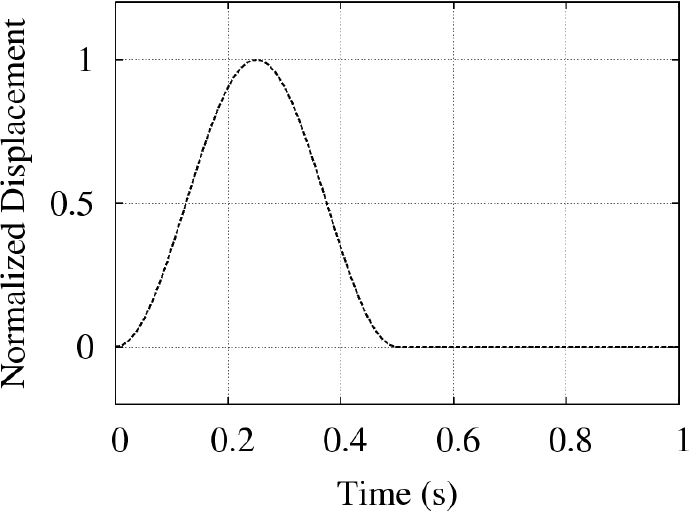
https://cdn.apub.kr/journalsite/sites/ksmer/2022-059-06/N0330590605/images/ksmer_59_06_05_F1.jpg

Fig. 1.

A pseudo-monochromatic source wavelet used in 1D modeling for measurement of velocity (Eq. (20)).

Fig. 2 shows the seismograms, which indicate that the wave quickly damps out with the distance. Figs. 2b, 2d, and 2f show amplified versions obtained by applying the gain function designed to compensate for the damping effect. In Figs. 2d and 2f, we observe severe dispersion, which makes it barely possible to measure the exact arrival time. Therefore, those cases are excluded from the velocity measurements. Fig. 3 shows the velocities measured for the three cases. When the frequency of the damping factor is the same as that of the source wavelet ((w_s, w_d ) = (4p, 4p) or (10p, 10p )), the measured velocity is almost identical to the analytical one (Figs. 3a and 3b). However, when the two frequencies are different ((w_s, w_d ) = (4p, 10p ), i.e., w_d is 2.5 times larger than w_s), the measured velocity deviates from the analytical one (Fig. 3c). Considering the discrepancy between the two frequencies, we recalculate the analytical velocity by increasing h to 2.5 times to its original value and display it in Fig. 3c. These results indicate that the representative frequency rather than the source frequency governs the damping effect of the SBC, and they should be the same. In Fig. 3, it is noted that the discrepancy becomes large as the damping factor increases. In this case, the wavelet changes due to the damping effect, and waves do not propagate as analytically expected. This tendency is dominant in the case of (w_s, w_d ) = (4p , 10p ) because the wavelet is more deformed by the discrepancy between the frequencies for the source wavelet and the damping factor.

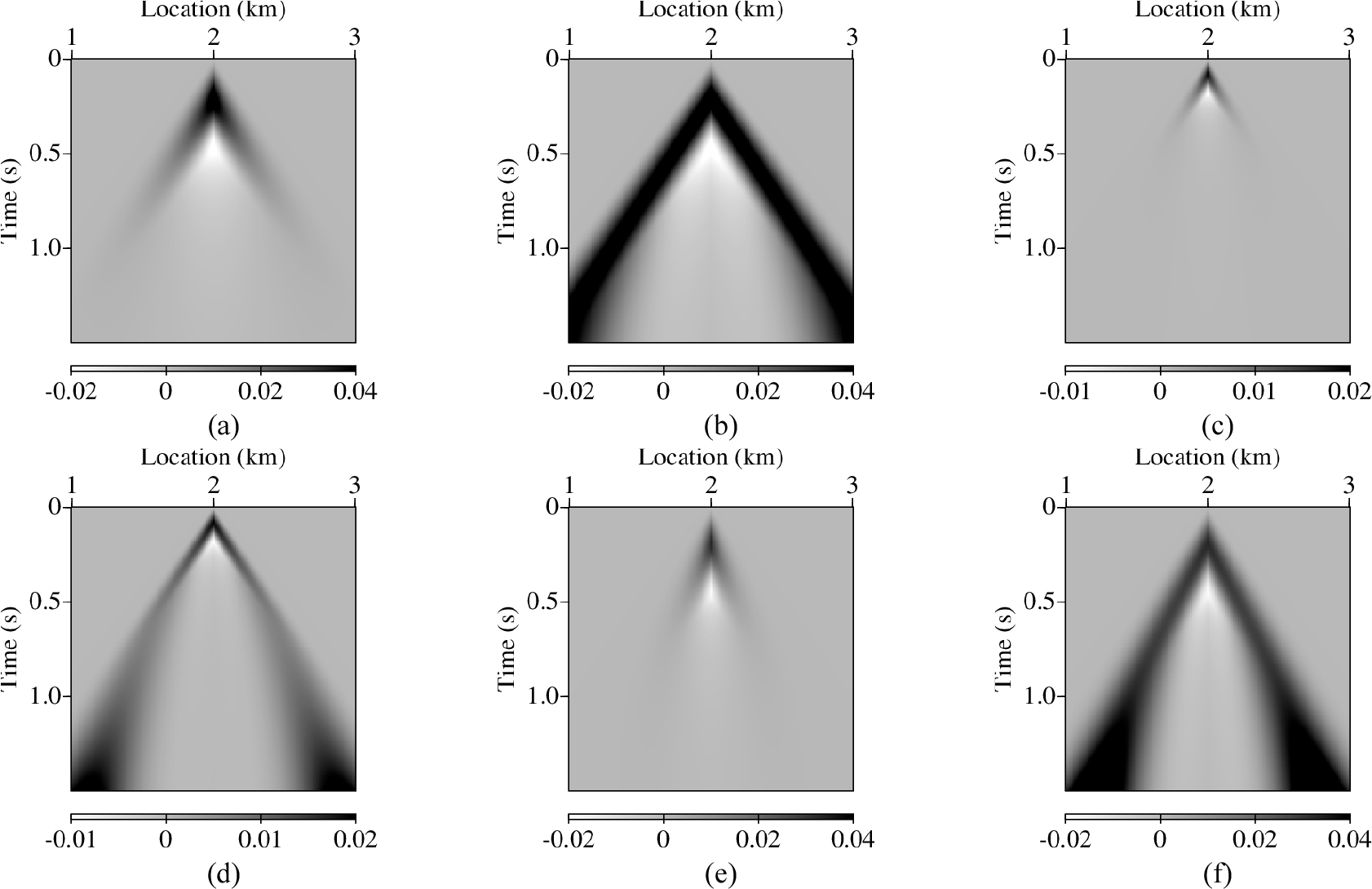
https://cdn.apub.kr/journalsite/sites/ksmer/2022-059-06/N0330590605/images/ksmer_59_06_05_F2.jpg

Fig. 2.

Seismograms obtained using time-domain modeling with an SBC for a constant damping factor of 0.5 and the 1D model for the frequency pairs of the source and damping factor of (a) (4p , 4p ), (c) (10p , 10p ), and (e) (4p , 10p ) and (b, d, f) their compensated version obtained using the gain function designed to cancel out the effect of the damping factor. The gain function compensates for the damping effect under the assumption that the peak amplitude decays exponentially.

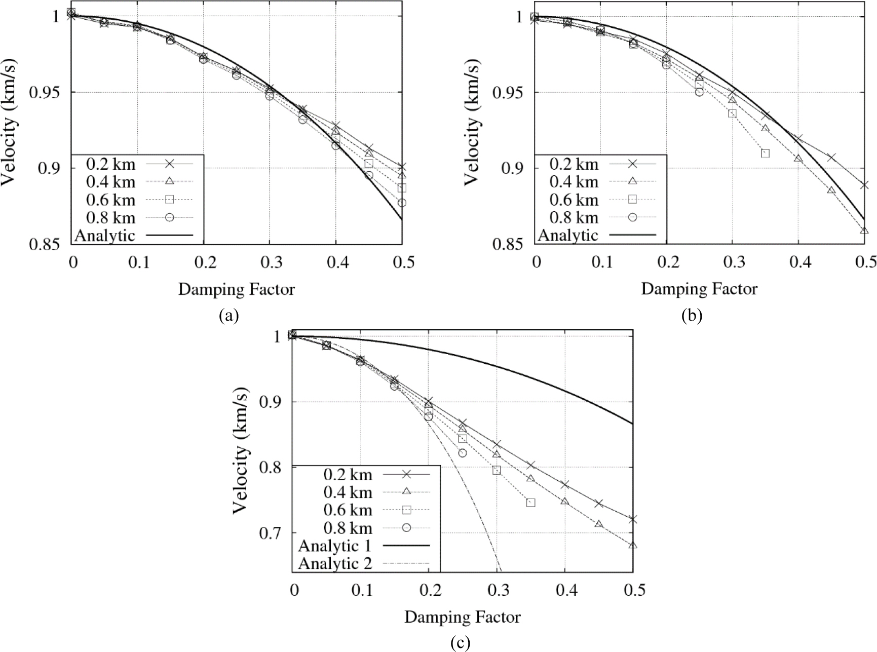
https://cdn.apub.kr/journalsite/sites/ksmer/2022-059-06/N0330590605/images/ksmer_59_06_05_F3.jpg

Fig. 3.

Wave velocities as a function of constant damping factors for the frequency pairs of the source and damping factor of (a) (4p , 4p ), (b) (10p , 10p ), and (c) (4p , 10p ). The bold solid lines indicate the analytical velocity derived by Eq. (12). The thin dashed line in (c) indicates the analytical velocity recalculated using 2.5h.

1D modeling with the SBC for multi-frequency waves

In general cases, seismic waves contain multi-frequency components. In the time domain, it is inefficient to apply different damping coefficients for each frequency component. Therefore, we inevitably use a representative frequency. We perform 1D modeling to examine how multi-frequency waves behave in the damping area when a representative frequency is used for the SBC in the time domain. Most of the parameters for modeling are the same as those of the monochromatic case shown in the previous subsection except for the source wavelet. The source wavelet comprises high- and low-frequency components for one period, which is given by

(21)

f (t) = \{\begin{cases} \frac{3 - 2 \cos (ω_{s} t) - \cos (4 ω_{s} t)}{2}, 0 \leq t \leq \frac{2 π}{ω_{s}} \\ 0, otherwise \end{cases},

as shown in Fig. 4. In this example, w_s is fixed to 4p. Similarly, it is acceptable to assume that the source wavelet has only two frequency components, i.e., 2 and 8 Hz

https://cdn.apub.kr/journalsite/sites/ksmer/2022-059-06/N0330590605/images/ksmer_59_06_05_F4.jpg

Fig. 4.

source wavelet comprising frequencies of 2 and 8 Hz, used for 1D modeling (Eq. 21).

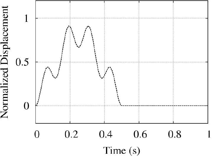
Fig. 5 shows modeling results obtained using a representative frequency of 4p and a damping factor (h ) of 0.5 for the SBC in the time domain: Fig. 5a is the original seismogram, and Fig. 5b is its amplified version with the gain function obtained in the same manner as Fig. 2b. The degrees of damping of the high- and low-frequency components look similar to each other. On the other hand, comparing Figs. 5c and 5d, which are the results for each frequency component under the same condition as in Fig. 5b, it is noted that the high-frequency component is slightly faster than the low-frequency component. These two tendencies conflict with the theoretical behavior described by Eq. (12).

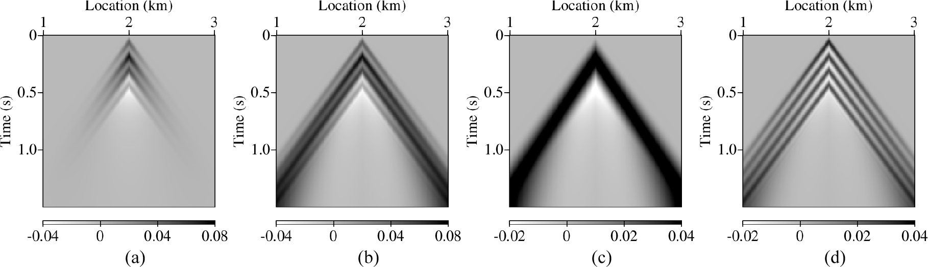
https://cdn.apub.kr/journalsite/sites/ksmer/2022-059-06/N0330590605/images/ksmer_59_06_05_F5.jpg

Fig. 5.

(a) Seismogram obtained using 1D time-domain modeling with the SBC, (b) its compensated version obtained using the gain function designed to cancel out the effect of the damping factor, and (c, d) the results for 2 and 8 Hz components under the same conditions as with (b). The gain function compensates for the damping effect under the assumption that the peak amplitude decays exponentially.

Now, we apply both the c-SBC and n-SBC to 1D modeling of the multi-frequency wave in the frequency domain. All the modeling parameters other than the domain are the same as those in Fig. 5. In this example, while the c-SBC still uses a representative frequency, i.e., the constant damping coefficient, the n-SBC applies different damping coefficients according to the frequency. Fig. 6 shows modeling results obtained by the c-SBC and n-SBC in the frequency domain. Figs. 6a and 6c are the original seismograms; Figs. 6b and 6d are their amplified versions obtained by applying the gain function as in Figs. 2b and 5b. Comparing Figs. 6 and 5, it is noted that while the c-SBC yields the same results (Figs. 6a and 6b) in both the time and frequency domains, the n-SBC gives different results (Figs. 6c and 6d), because n-SBC preferentially damps out high-frequency waves, which conforms to Eq. (12).

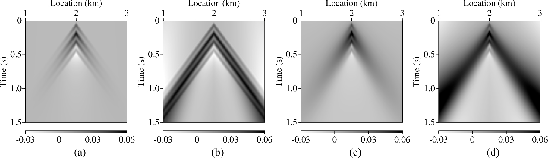
https://cdn.apub.kr/journalsite/sites/ksmer/2022-059-06/N0330590605/images/ksmer_59_06_05_F6.jpg

Fig. 6.

Seismograms obtained using 1D frequency-domain modeling with the (a) c-SBC and (c) n-SBC and (b, d) their compensated versions obtained using the gain function designed to cancel out the effect of the damping factor. The gain function compensates for the damping effect under the assumption that the peak amplitude decays exponentially.

Comparison of the SBCs and PML for 2D modeling

To estimate the performance of the n-SBC, we apply the aforementioned two SBCs and PML to 2D homogeneous model as a boundary condition. The dimension of the model is 2 km × 2 km consisting of 10 meter-sized grids, and its P-wave velocity is 3 km/s. A Ricker wavelet with a peak frequency of 11.8 Hz is applied at the center of the model. The boundary conditions are applied to the left, right, and bottom boundaries, while the top remains as a free surface. Although the boundary conditions are applied, artificial reflections are not perfectly suppressed, and some energy is still reflected at the damping area. We classify artificial reflections into two types. The first type is generated due to the change of the damping factor in the damping area, resulting in the variation of physical properties between grid points, which will be called “type-1 reflection”. The second type is the reflection of remaining energy at the outer boundary of the damping area, which will be called “type-2 reflection”. To evaluate the performance of the three boundary conditions, we need to separate and quantify the type-1 and type-2 reflections. To do so, we conduct modeling to get three seismograms. The first one is the full seismogram containing both the type-1 and type-2 reflections. The second one is the seismogram with only the type-1 reflection, which is obtained with a large damping area using 150 grids for each direction such that the type-2 reflection does not have enough time to return to the modeling regions. The last one is free from artificial reflections, which is obtained by performing modeling for a large model without any boundary conditions such that both the type-1 and type-2 reflections do not return to the receivers during the recording. The procedure for separating the type-1 and type-2 reflections is summarized as follows: 1) We first extract a residual seismogram containing both the type-1 and type-2 reflections by subtracting the artificial reflection-free seismogram from the full seismogram; 2) We obtain another residual seismogram containing only the type-1 reflection in a similar manner to that applied in the first step; 3) We subtract the result of the second step from that of the first step to extract only the type-2 reflection. To estimate errors, we sum all the absolute values of the residual seismograms obtained in the second and last stages. As shown in Fig. 7, artificial reflections in seismograms emerge in the form of X-cross shape with the bottom bar. We set an adequate time window that only contains one reflection.

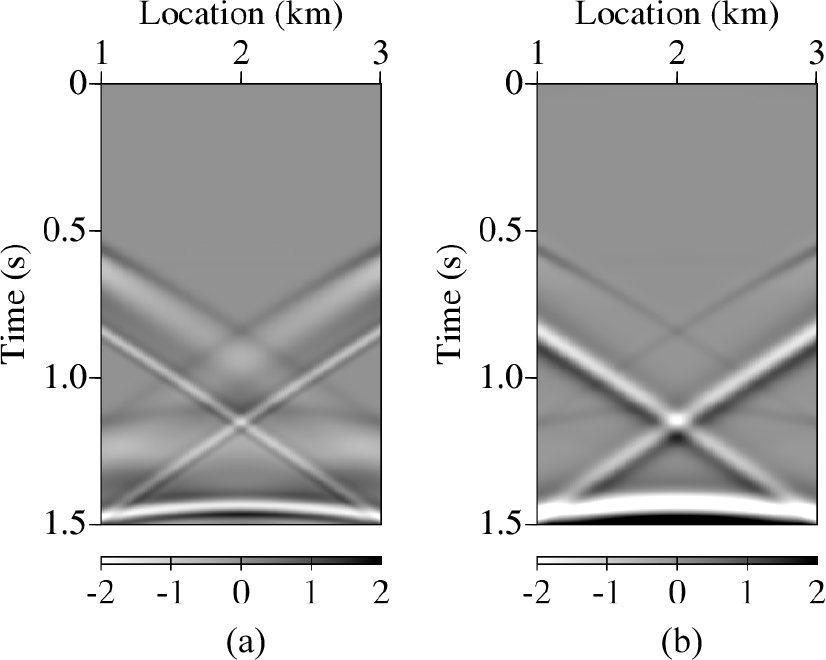
https://cdn.apub.kr/journalsite/sites/ksmer/2022-059-06/N0330590605/images/ksmer_59_06_05_F7.jpg

Fig. 7.

Residual seismograms obtained by subtracting the reflection-free seismogram from the full seismogram containing both type-1 and type-2 reflections. (a) and (b) are the results of the c-SBC and n-SBC, respectively. (a) contains more type-1 reflections and fewer type-2 reflections. The type-2 reflections in (b) are lengthened due to preferential suppression of high-frequency components by the n-SBC.

In this experiment, we assign 50 grids in each direction for the damping area of both the SBCs. The damping factor increases in quadratic, cubic, or quartic manners from 0 at the inner boundary to 0.5 or 1 at the outer boundary. We exclude a linear case from the consideration because an abrupt change near the inner boundary generates excessive type-1 reflections. For the damping area of the PML, 20 and 50 grids are used, which will be named the “PML-20” and “PML-50”, respectively. The brief theoretical basis of the PML is provided in Appendix B. Table 1 includes the amount of type-1 and type-2 reflections of the SBCs with various damping factors and the PMLs. Observations from the modeling results obtained using the n-SBC and c-SBC are summarized as follows:

1) The damping factor increasing in a higher order does not suppress the type-1 reflections well. In this case, the damping factor changes slightly near the inner boundary but increases rapidly with the distance from the inner boundary. The type-1 reflections are generated throughout the whole damping area due to the abrupt increase of the damping factor;

2) The type-2 reflection becomes more dominant as the damping factor increases in a higher order, because the damping effect is not large enough to damp out waves sufficiently. Consider that the multiplication of small values (< 1) yields smaller values;

3) The n-SBC generates fewer type-1 reflections and more type-2 reflections than the c-SBC. Because the n-SBC damps high-frequency components preferentially but does not sufficiently suppress low-frequency components, an amount of low-frequency energy is reflected at the outer boundary and returns to the modeling area. Accordingly, the low-frequency components are dominant in the type-2 reflection as shown in Fig. 7.

Table 1.

The amount of the type-1 and type-2 reflections in seismograms obtained with the n-SBC, c-SBC, vg-SBC, PML-20, and PML-50. The SBCs are subdivided into six classes according to the maximum damping factor at the outer boundary and the increasing order of the damping factor

ABC	Type of reflection	Max η
		0.5			1
		Increasing order
		2nd	3rd	4th	2nd	3rd	4th
n-SBC	Type-1	8.49	8.49	13.97	21.45	19.60	27.00
n-SBC	Type-2	64.15	111.92	163.33	15.55	29.39	47.39
c-SBC	Type-1	32.90	29.23	33.82	61.88	48.59	51.28
c-SBC	Type-2	22.68	60.56	110.02	1.00	4.55	12.97
vg-SBC	Type-1	6.84	2.19	1.13	16.00	5.14	2.51
vg-SBC	Type-2	2.22	3.72	5.55	0.42	0.73	1.13
PML-20	Type-1	9.17
PML-20	Type-2	1.16
PML-50	Type-1	0.32
PML-50	Type-2	1.28

Considering the first and second observations together, the quadratic increase of the damping factor is the most adequate for both SBCs. Compared with the PML-20, the best case of the n-SBC (with an h of 1) generates 2 times more type-1 reflections and is not free from type-2 reflections. However, the n-SBC is easy to be simulated and computationally efficient compared to the PML. This aspect is analyzed in the upcoming subsection.

The best case of the n-SBC with 50 grids causes almost 4 times the total error generated by the PML-20, which indicates that the SBC requires more grids for the damping area to suppress artificial reflections to the same extent. However, it is not feasible to increase the number of grids for the damping area, because it increases computational overhead.

Variable grid method for the n-SBC modeling

To enhance the applicability of the SBC, we suggest using the variable grid method, in which the grid size gradually increases towards the outer boundary. The idea of applying a coarser grid with the distance from the source has been widely used in the modeling of CSEM or MT surveys (Nam et al., 2007; Plessix et al., 2007), which use logarithmically scaled grids. In the literature, we can find that the similar idea was applied to seismic modeling and inversion (Choi et al., 2014) and other optimization-based multi-grid methods were proposed (Pitarka, 1999; Hayashi et al., 2001; Wu and Harris, 2004). Because coarse grids can cause numerical dispersion of the high-frequency components (Mullen and Belyschko, 1982), it is needed to apply the optimization technique to properly manage the operators. However, the n-SBC is robust against numerical dispersion without additional treatments, because it damps out high-frequency components preferentially, which plays a role in lowering the peak frequency of waves as waves propagate through the damping area. Therefore, we can apply the variable grid method to the n-SBC (‘vg-SBC’) with a little burden. In contrast, with the variable grid method, the c-SBC is vulnerable to numerical dispersion, because it damps out all frequency components to a similar degree and does not lower the peak frequency. The grid size quadratically increases beginning at the inner boundary to 5 times of the original grid size at the outer boundary. Table 1 includes the amount of type-1 and type-2 reflections of the vg-SBC. In Table 1, it is noted that the vg-SBC shows quite enhanced performance compared with both the n-SBC and c-SBC. Specifically, the vg-SBC, whose damping factor increases to 1 in a quartic manner, shows comparable performance to the PML-50. While the n-SBC generates the type-1 reflection throughout the damping area and the type-2 reflection as well, the vg-SBC generates some type-1 reflections near the inner boundary and significantly reduces type-2 reflections. However, if we excessively increase the grid size, the vg-SBC may suffer from numerical dispersion. Fig. 8 shows the result obtained using the vg-SBC, in which the grid size gradually increases to 5 or 10 times the original grid size at the outer boundary. In Fig. 8b, we observe that the vg-SBC also suffers from numerical dispersion with a carelessly large increase in grid size.

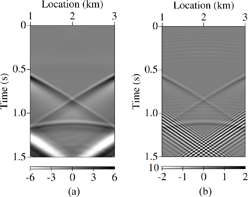
https://cdn.apub.kr/journalsite/sites/ksmer/2022-059-06/N0330590605/images/ksmer_59_06_05_F8.jpg

Fig. 8.

Residual seismograms obtained by modeling with the vg-SBC, where grid size increases to (a) 5 times and (b) 10 times its original size at the outer boundary. In (b), severe numerical dispersion is observed. Note the difference of the scales; (b) contains more artificial reflections than (a) due to numerical dispersion.

Comparison of the SBCs and PML for computational efficiency

In Table 1, it is noted that both the c-SBC and n-SBC generate more artificial reflections than the PML-20, even though both SBCs use a 2.5 times broader damping area than the PML-20. The n-SBC with 70 grids generates a similar degree of artificial reflections to PML-20 (8.72 type-1 and 3.46 type-2 reflections). In other words, the n-SBC requires a broader damping area than PML to show a similar degree of performance. We organize the computational costs of the SBCs and PML in Tables 2 and 3, in which both the n-SBC and c-SBC are categorized as the SBC because their aspects are almost identical. The geometry for modeling is the same as that of the 2D examples, but the base model dimension exponentially increases from 200×200 to 1600×1600. In Tables 2 and 3, similar aspects for both computational cost and memory overhead are observed. If the dimension of the padded areas of the SBC and PML are identical, the SBC is computationally efficient than the PML, and if the padded area of the SBC is broader than that of the PML, overheads for the broader padded area dominates the computational inefficiency of the PML when the base model is relatively small, but it reverses as the model gets large.

Table 2.

The computing times (in seconds) of the SBC, vg-SBC, PML-20, and PML-50 according to the base model dimension for a single frequency component

ABC	Base model dimension
ABC	200×200	400×400	800×800	1600×1600
SBC	0.604	2.127	8.120	28.150
vg-SBC	0.683	2.647	10.488	36.957
PML-20	0.479	2.306	8.933	34.548
PML-50	0.691	2.806	10.870	38.866

Table 3.

The memory overheads per the number of grid nodes (in bytes) of the SBC, vg-SBC, PML-20, and PML-50 with respect to the base model dimension. Averages are calculated geometrically. The modeling is conducted in single precision format.

ABC	Base model dimension				Average
ABC	200×200	400×400	800×800	1600×1600	Average
SBC	73.602	36.413	19.605	11.651	27.972
vg-SBC	148.458	92.643	67.418	55.482	84.691
PML-20	119.110	94.881	83.271	77.593	92.440
PML-50	200.764	131.964	100.869	86.155	123.181

The SBC is efficient in terms of the computational cost for two reasons. Consider that the SBC modifies the mass term, whereas the PML changes the stiffness term. In modeling with the FDM, the SBC changes only diagonal entries in the matrix of the modeling operator, but the PML changes off-diagonal ones asymmetrically. Accordingly, the SBC preserves the symmetry of the modeling operator, but the PML makes the modeling operator asymmetric. The algorithm for solving the symmetric matrix equation is more efficient than that for the asymmetric case, which is adopted in Intel MKL PARDISO. Furthermore, because the SBC replaces only the w² term of the basic wave equation, there is almost no overhead for composing modeling operator with the SBC.

SBC requires less computer memory than the PML due to two aspects. First, the SBC needs to save only the lower-or upper-triangular part of the matrix because its modeling operator is symmetrical. Second, the SBC requires only one extra parameter, i.e., the damping factor, while the PML requires two parameters and one more optional parameter for each axis. For instance, for 2D modeling, the PML requires six parameters, while the SBC requires one parameter. In summary, the SBC has advantages over the PML when considering the computational efficiency, specifically for large-sized models.

Unfortunately, when considering the vg-SBC, the advantages of the SBC resulting from symmetry are no longer viable. In FDM modeling, introducing the variable grid method ruins the symmetry of the modeling operator. However, the vg-SBC requires the same amount of computation for composing the modeling matrix as the SBC; thus, the vg-SBC is still faster than the PML-50, as shown in Table 2. Furthermore, although the vg-SBC requires one more extra parameter (i.e., the grid size) for each axis compared with the SBC, the PML still requires more memory than the vg-SBC. Therefore, the vg-SBC has some advantages compared with the PML in terms of computational cost and memory efficiency.

Discussion

In this study, we proposed the new governing equation of the SBC and provided various examples to explain its characteristics. Unlike the c-SBC, the n-SBC preferentially removes high frequencies, which makes it possible to implement the vg-SBC using the variable grid, which performs similarly to the PML. Furthermore, we compared the SBCs and the PML in terms of the computational cost and showed that the SBCs have computational advantages over the PML. In this section, we will discuss the points to be noted and the improvement related to the study.

Although all modeling in this study was implemented with the FDM, another modeling method called the finite-element method (FEM), which composes a solution by approximating the solution space through a set of basis functions, is also widely used for seismic modeling as well (Marfurt, 1984; Serón et al., 1990). When performing frequency-domain modeling with the FEM, the asymmetry issue hindering the performance of the PML or the vg-SBC can be resolved because the matrix system preserves symmetry in most cases due to the characteristic of the FEM.

Since the PML applies the damping effect according to the direction of wave propagation in space, it may not work properly in anisotropic media. This is because the directions of the wave propagation and group velocity may be opposite under certain anisotropic conditions. However, the SBC is free from this problem because it applies a damping effect regardless of the direction of the wave propagation. Therefore, it may be necessary to research the behavior of the SBC in anisotropic media to overcome the issue concerned with the PML. To do so, it is firstly required to check how for the SBC to be applied in elastic media for isotropic and anisotropic cases. Considering the characteristics of SBC, it is simple to apply SBC in elastic media by replacing the w² term. Although only the results for acoustic media were presented in this paper, the SBC can be applied to elastic media in the same manner.

Further improvement can be done for the vg-SBC. We fixed the grid size over all the frequencies used for modeling with the vg-SBC. However, there are no limitations to use different grid sizes for different frequencies, which makes it possible to assign an appropriate grid for modeling with the vg-SBC in the frequency domain. As shown in Fig. 8, an excessively large grid size can cause dispersion and degrades the modeling performance, which indicates that not exceeding an appropriate grid size for each frequency is critical for the vg-SBC. By assigning a proper grid size for each frequency which maximizes the intensity of the damping effect while suppressing the dispersion, the performance of the vg-SBC may be further improved.

Conclusions

Since the conventional SBC was designed to damp out waves in the padded area of a given model, it has not been discussed academically or used practically due to its low applicability. In this study, we established the new governing equation of the SBC and derived its analytical solution, thus showing that the new governing equation is similar to that for describing intrinsic attenuation in viscoelastic media. The 1D examples showed that the c-SBC does not appropriately describe the theoretical behavior of wave propagation in damped media, which is because the c-SBC applies a fixed damping coefficient irrespective of the frequency. In contrast, the n-SBC fixes the damping factor, which changes the damping coefficient according to the frequency. In the time domain, it is not practical to apply the frequency-dependent damping coefficient, but it is easy to be done in the frequency domain because the modeling is performed for each frequency. The 2D examples showed that the n-SBC has some advantages compared with the c-SBC, but the SBCs require a broader padded area than the PML to show a similar degree of performance. However, for FDM modeling, the SBC has advantages over the PML with respect to the computational efficiency, specifically for large-sized models. On the other hand, considering that the n-SBC preferentially suppresses the high-frequency components and lowers the dominant frequency of the wave, we proposed combining the n-SBC with the variable grid method. Numerical examples showed that the vg-SBC enhances the suppression of artificial reflections and becomes comparable to the PML while preserving its computational efficiency to some extent.

Appendix A. Modeling of the new SBC with attenuation

To prevent the wrap-around effect in frequency-domain modeling, we use the complex frequency (w + ia ), whose imaginary part plays a role in giving an attenuation effect, and then restore the attenuation effect in the recording phase. However, the n-SBC cannot adopt the complex frequency by just replacing w with w + ia. In this section, the method of applying the n-SBC with the complex frequency is derived following the method employed by Song and Williamson (1995).

Adding the source term into Eq. (8) yields

(A.1)

(\nabla^{2} - \frac{1}{v^{2}} (D^{2} + 2 η ω D)) u = - s (t) δ (r - r_{0}) δ (t - t_{0}),

where s is the source function; D indicates the time derivate operator; d indicates the Dirac delta function; r₀ and t₀ indicate the time and location of source, respectively. Let $u (t) = e^{α t} u' (t)$ be the solution of Eq. (A.1), where $u' (t)$ is the solution with the attenuation effect. Substituting $u (t) = e^{α t} u' (t)$ into Eq. (A.1) yields

(A.2)

(\nabla^{2} - \frac{1}{v^{2}} (D^{2} + 2 η ω D)) (e^{α t} u') = - s (t) δ (r - r_{0}) δ (t - t_{0}),

By dividing Eq. (A.2) by $e^{α t}$ , we obtain

(A.3)

(\nabla^{2} - \frac{1}{v^{2}} (D^{2} + 2 α D + a^{2} + 2 η ω D + 2 η ω α)) u' = - e^{α t} s (t) δ (r - r_{0}) δ (t - t_{0}),

and taking the Fourier transform of Eq. (A.3) gives

(A.4)

(\nabla^{2} + \frac{1}{v^{2}} ((1 - 2 i η) ω^{2} - 2 (i + η) α ω - a^{2}) \tilde{u}' = - e^{- α t} \tilde{s} (t) δ (r - r_{0}) δ (t - t_{0}) .

The basic wave equation can be converted to a similar form with Eq. (A.4), which is given by

(A.5)

(\nabla^{2} + \frac{ω^{2}}{v^{2}}) \tilde{u}' = - \tilde{s} (t) δ (r - r_{0}) δ (t - t_{0}) .

When comparing Eq. (A.4) with Eq. (A.5), it is noted that Eq. (A.4) can be obtained by replacing

(A.6)

ω^{2} \to (1 - 2 i η) ω^{2} - 2 (i + η) α ω - a^{2} .

In contrast, the c-SBC with the complex frequency does not require this kind of approach and can easily be applied by replacing w of Eq. (19) with w + ia.

Appendix B. Acoustic modeling with the PML

The analytic expression of waves $A e^{i (k x + - ω t)}$ is converted to $A e^{- f (x) k} e^{i (k x \pm ω t)}$ replacing the spatial variable x with x + if(x), where the additional term represent the damping effect in the spatial directions. The PML incorporates the damping effect by expanding the spatial coordinate to the imaginary direction. When the spatial variable x is replaced with x + if(x), the spatial-differential operator is converted as follows:

(B.1)

\frac{\partial}{\partial x} \to \frac{\partial}{\partial (x + i f (x))} = \frac{\partial}{\partial x} \frac{1}{1 + i f' (x)} = \frac{\partial}{\partial x} \frac{i ω}{i ω - ω f' (x)} .

In practice, $ω f' (x)$ , indicating the amount of the damping effect, is assigned like a model property in the padded area whose form in practice is suggested by Collino and Tsogka (2001) in acoustic modeling as follows:

(B.2)

d (x) = ω f' (x) = \ln (1000) \frac{3 v (x)}{2 δ} {(\frac{x}{δ})}^{2},

where v(x) is the wave velocity and d indicates the width of the padded area. Starting from Eq. (B.1), we can incorporate the damping effect into the 2D frequency-domain acoustic wave equation. For convenience, we simplify the last part of Eq. (B.1) with new functions as follows:

(B.3)

\frac{\partial}{\partial x} \frac{i ω}{i ω - ω f_{x}^{'} (x)} = S_{x} (x) \frac{\partial}{\partial x} \frac{\partial}{\partial z} \frac{i ω}{i ω - ω f_{z}^{'} (z)} = S_{z} (z) \frac{\partial}{\partial z},

where z is another spatial variable for the 2D case. Then the 2D frequency-domain acoustic wave equation is converted with the modified spatial-differential operators as follows:

(B.4)

- \frac{ω^{2}}{v^{2}} \tilde{u} = \frac{\partial^{2} \tilde{u}}{\partial x^{2}} + \frac{\partial^{2} \tilde{u}}{\partial z^{2}} \to - \frac{ω^{2}}{v^{2}} \tilde{u} = S_{x} \frac{\partial}{\partial x} (S_{x} \frac{\partial u}{\partial x}) + S_{z} \frac{\partial}{\partial z} (S_{z} \frac{\partial u}{\partial z}) = S_{x}^{2} \frac{\partial^{2} \tilde{u}}{\partial x^{2}} + S_{x} S'_{x} \frac{\partial u}{\partial x} + S_{z}^{2} \frac{\partial^{2} \tilde{u}}{\partial z^{2}} + S_{z} S'_{z} \frac{\partial u}{\partial z},

where S_x and S_z are defined as Eqs. (B.2) and (B.3) in the padded area.

Acknowledgements

This work is supported by the National Research Foundation of Korea (NRF) grant funded by the Ministry of Science & ICT, Republic of Korea (MSIT) (No. 2021R1A2C1092820) and the Development of high-performance monitoring technology for marine CO₂ storage of the Korea Institute of Energy Technology Evaluation and Planning (KETEP) granted financial resource from the Ministry of Trade, Industry & Energy, Republic of Korea (MOTIE) (No. 20226A10100030).

References

Aki, K., and Richards, P.G., 2002. Quantitative Seismology (2nd Ed.), University Science Books, New York, USA, p.161-177.

Becache, E., Fauqueux, S., and Joly, P., 2003. Stability of perfectly matched layers, group velocities and anisotropic waves, Journal of Computational Physics, 188, p.399-433. 10.1016/S0021-9991(03)00184-0

Berenger, J.P., 1994. A perfectly matched layer for the absorption of electromagnetic waves, Journal of Computational Physics, 114(2), p.185-200. 10.1006/jcph.1994.1159

Cerjan, C., Kosloff, D., Kosloff, R., and Reshef, M., 1985. A nonreflecting boundary condition for discrete acoustic and elastic wave equations, Geophysics, 50(4), p.705-708. 10.1190/1.1441945

Chang, W.F. and McMechan, G.A., 1989. Absorbing boundary conditions for 3-D acoustic and elastic finite-difference calculations, Bulletin of the Seismological Society of America, 79(1), p.211-218. 10.1785/BSSA0790010211

Choi, S., Min, D.J., Oh, J.W., Chung, W., Ha, W., and Shin, C., 2014. Frequency-domain acoustic and elastic modeling and waveform inversion in the logarithmic grid set, Journal of Seismic Exploration, 23(2), p.103-130.

Clayton, R. and Engquist, B., 1977. Absorbing boundary conditions for acoustic and elastic wave equations, Bulletin of the Seismological Society of America, 67(6), p.1529-1540. 10.1785/BSSA0670061529

Collino, F. and Tsogka, C., 2001. Application of the perfectly matched absorbing layer model to the linear elastodynamic problem in anisotropic heterogeneous media, Geophysics, 66(1), p.294-307. 10.1190/1.1444908

Frankel, A. and Wennerberg, L., 1987. Energy-flux model of seismic coda: separation of scattering and intrinsic attenuation, Bulletin of the Seismological Society of America, 77(4), p.1223-1251. 10.1785/BSSA0770041223

Hagstrom, T., Givoli, D., Rabinovich, D., and Bielak, J., 2014. The double absorbing boundary method, Journal of Computational Physics, 259, p.220-241. 10.1016/j.jcp.2013.11.025

Hayashi, K., Burns, D.R., and Toksöz, M.N., 2001. Discontinuous-grid finite-difference seismic modeling including surface topography, Bulletin of the Seismological Society of America, 91(6), p.1750-1764. 10.1785/0120000024

Heidari, A.H. and Guddati, M.N., 2006. Highly accurate absorbing boundary conditions for wide-angle wave equations, Geophysics, 71(3), p.S85-S97. 10.1190/1.2192914

Higdon, R.L., 1991. Absorbing boundary conditions for elastic waves, Geophysics, 56(2), p.231-241. 10.1190/1.1443035

Ikelle, L.T. and Amundsen, L., 2005. Introduction to Petroleum Seismology, Vol. 12 SEG Books, Tulsa, USA, p.598-606. 10.1190/1.9781560801702

Jo, C.H., Shin, C., and Suh, J.H., 1996. An optimal 9-point, finite-difference, frequency-space, 2D scalar wave extrapolator, Geophysics, 61(2), p.529-537. 10.1190/1.1443979

Keys, R.G., 1985. Absorbing boundary conditions for acoustic media, Geophysics, 50(6), p.892-902. 10.1190/1.1441969

Liao, Q. and McMechan, G.A., 1993. 2D pseudo-spectral viscoelastic modeling in a distributed-memory multi-processor computer, Bulletin of the Seismological Society of America, 83(5), p.1345-1354. 10.1785/BSSA0830051345

Liu, Y. and Sen, M.K., 2010. A hybrid scheme for absorbing edge reflections in numerical modeling of wave propagation, Geophysics, 75(2), p.A1-A6. 10.1190/1.3295447

Marfurt, K.J., 1984. Accuracy of finite-difference and finite-element modeling of the scalar and elastic wave equations, Geophysics, 49(5), p.533-549. 10.1190/1.1441689

Métivier, L., Brossier, R., Labbé, S., Operto, S., and Virieux, J., 2014. A robust absorbing layer method for anisotropic seismic wave modeling, Journal of Computational Physics, 279, p.218-240. 10.1016/j.jcp.2014.09.007

Mullen, R. and Belytschko, T., 1982. Dispersion analysis of finite element semidiscretizations of the two-dimensional wave equation, International Journal for Numerical Methods in Engineering, 18(1), p.11-29. 10.1002/nme.1620180103

Nam, M.J., Kim, H.J., Song, Y., Lee, T.J., Son, J.S., and Suh, J.H., 2007. 3D magnetotelluric modelling including surface topography, Geophysical Prospecting, 55(2), p.277-287. 10.1111/j.1365-2478.2007.00614.x

Pitarka, A., 1999. 3D elastic finite-difference modeling of seismic motion using staggered grids with nonuniform spacing, Bulletin of the Seismological Society of America, 89(1), p.54-68. 10.1785/BSSA0890010054

Plessix, R.E., Darnet, M., and Mulder, W.A., 2007. An approach for 3D multisource, multifrequency CSEM modeling, Geophysics, 72(5), p.SM177-SM184. 10.1190/1.2744234

Potter, T., Shragge, J., and Lumley, D., 2019. Performance and stability of the double absorbing boundary method for acoustic-wave propagation, Geophysics, 84(2), p.T59-T72. 10.1190/geo2018-0161.1

Rabinovich, D., Givoli, D., Bielak, J., and Hagstrom, T., 2017. The Double Absorbing Boundary method for a class of anisotropic elastic media, Computer Methods in Applied Mechanics and Engineering, 315, p.190-221. 10.1016/j.cma.2016.10.035

Ren, Z. and Liu, Y., 2013. A hybrid absorbing boundary condition for frequency-domain finite-difference modelling, Journal of Geophysics and Engineering, 10(5), p.16-31. 10.1088/1742-2132/10/5/054003

Reynolds, A.C., 1978. Boundary conditions for the numerical solution of wave propagation problems, Geophysics, 43(6), p.1099-1110. 10.1190/1.1440881

Schenk, O., Gärtner, K., and Fichtner, W., 2000. Efficient sparse LU factorization with left-right looking strategy on shared memory multiprocessors, BIT Numerical Mathematics, 40(1), p.158-176. 10.1023/A:1022326604210

Schenk, O. and Gärtner, K., 2004. Solving unsymmetric sparse systems of linear equations with PARDISO, Future Generation Computer Systems, 20, p.475-487. 10.1016/j.future.2003.07.011

Serón, F.J., Sanz, F.J., Kindelan, M., and Badal, J.I., 1990. Finite‐element method for elastic wave propagation, Communications in Applied Numerical Methods, 6(5), p.359-368. 10.1002/cnm.1630060505

Shin, C., 1995. Sponge boundary condition for frequency-domain modeling, Geophysics, 60(6), p.1870-1874. 10.1190/1.1443918

Smith, W.D., 1974. A nonreflecting plane boundary for wave propagation problems, Journal of Computational Physics, 15(4), p.492-503. 10.1016/0021-9991(74)90075-8

Song, Z.M. and Williamson, P.R., 1995. Frequency-domain acoustic-wave modeling and inversion of crosshole data: Part I-2.5-D modeling method, Geophysics, 60(3), p.784- 795. 10.1190/1.1443817

Virieux, J., 1984. SH-wave propagation in heterogeneous media: Velocity-stress finite-difference method, Geophysics, 49(11), p.1933-1942. 10.1190/1.1441605

Virieux, J., 1986. P-SV wave propagation in heterogeneous media: Velocity-stress finite-difference method, Geophysics, 51(4), p.889-901. 10.1190/1.1442147

Wu, C. and Harris, J.M., 2004. An optimized variable-grid finite-difference method for seismic forward modeling, Journal of Seismic Exploration, 12(4), p.343-353.

Zhou, H. and McMechan G.A., 2000. Rigorous absorbing boundary conditions for 3-D one-way wave extrapolation, Geophysics, 65(2), p.638-645. 10.1190/1.1444760

Journal of the Korean Society of Mineral and Energy Resources Engineers ISSN:2288-0291(Print) 2288-2790(Online) 한국자원공학회지

Preview

Seismic Wave Modeling with an Improved Sponge Boundary Condition Considering Viscoelastic Behavior

ABSTRACT

MAIN

(1)

(2)

(3)

(4)

(5)

(6)

(7)

(8)

(9)

(10)

(11)

(12)

(13)

(14)

(15)

(16)

(17)

(18)

(19)

(20)

Fig. 1.

A pseudo-monochromatic source wavelet used in 1D modeling for measurement of velocity (Eq. (20)).

Fig. 2.

Fig. 3.

(21)

Fig. 4.

source wavelet comprising frequencies of 2 and 8 Hz, used for 1D modeling (Eq. 21).

Fig. 5.

Fig. 6.

Fig. 7.

Table 1.

The amount of the type-1 and type-2 reflections in seismograms obtained with the n-SBC, c-SBC, vg-SBC, PML-20, and PML-50. The SBCs are subdivided into six classes according to the maximum damping factor at the outer boundary and the increasing order of the damping factor

Fig. 8.

Table 2.

The computing times (in seconds) of the SBC, vg-SBC, PML-20, and PML-50 according to the base model dimension for a single frequency component

Table 3.

The memory overheads per the number of grid nodes (in bytes) of the SBC, vg-SBC, PML-20, and PML-50 with respect to the base model dimension. Averages are calculated geometrically. The modeling is conducted in single precision format.

(A.1)

(A.2)

(A.3)

(A.4)

(A.5)

(A.6)

(B.1)

(B.2)

(B.3)

(B.4)

Acknowledgements

References