

Introduction
UBGH2-6 site and space discretization
Forward simulation
Deep Learning Modeling
Sensitivity Analysis - Model Architecture
Results & Discussion
Conclusion
Introduction
Modeling of gas hydrate deposits entails high computational costs due to the strongly nonlinear and tightly coupled nature of fluid transport and thermal flow processes (Moridis, 2003; Rutqvist and Moridis, 2009; Rutqvist et al., 2009; Kim et al., 2012a; Yoon et al., 2021; Zhang et al., 2023). For instance, depressurization leads to gas hydrate dissociation into gas and water, accompanied by a simultaneous temperature drop owing to the endothermic nature of the reaction. These phase changes subsequently influence flow regimes, altering porosity and permeability and thus affecting the pressure field (Rutqvist and Moridis, 2009; Kim et al., 2012b; White et al., 2020; Kim and Lee, 2024).
Numerical simulation of gas production from UBGH2-6, a gas hydrate deposit located in the Ulleung Basin, South Korea, poses considerable challenges and can require extensive computational time, especially under complex production scenarios (Moridis et al., 2013; Kim et al., 2017; Lee et al., 2021; Yoon et al., 2021; Yoon et al., 2022; Yoon et al., 2024). For example, simulations involving periodic depressurization demand substantially more computational resources compared to constant depressurization cases (Yoon et al., 2021). Consequently, sudden changes in bottom hole pressure (BHP) driven by safety controls can preclude timely productivity predictions when relying exclusively on full-physics simulations. Therefore, it is imperative to develop alternative approaches that can deliver rapid and reliable prediction results to optimize gas production while mitigating operational risks in the field.
Machine learning (ML) has emerged as a powerful modeling strategy, offering significant reductions in computational cost while maintaining high predictive accuracy (Sarkar et al., 2025). Recent studies have successfully applied ML techniques to a variety of reservoir engineering challenges, including optimization of well spacing and completions (Wang and Sun, 2020), production forecasting (Chaikine and Gates, 2021), hydraulic fracture design (Sarkar et al., 2025), and leakage risk assessment (Baek et al., 2023; Baek et al., 2025). For problems related to gas hydrates, Park et al. (2022) applied multiple ML algorithms—such as random forest (RF), multi-layer perceptron, convolutional neural networks (CNN), and recurrent neural networks (RNN)—to predict mineral compositions of gas hydrate sediments from the Ulleung Basin, Korea, based on X-ray diffraction (XRD) data.
Ji et al. (2022) generated compressional wave velocity predictions from well-logging data (e.g., gamma-ray and neutron porosity) obtained from the UBGH area in the East Sea, utilizing artificial neural networks (ANN) and long short-term memory (LSTM) models. Their study also conducted sensitivity analyses on input log combinations and model architecture to optimize performance. Wu and Li (2025) compared attention-based models, ResNet, and simple CNNs to identify the occurrence and depth of natural gas hydrates using attributes such as P-wave velocity, resistivity, and density measurements. Patel and Jana (2024) employed various ML models—including RF, gradient boosting (GB), extra trees (ET), and decision trees (DT)—to model gas hydrate formation and growth dynamics derived from laboratory experimental data, benchmarking results against fundamental thermokinetic models. Park et al. (2021) systematically reviewed and compiled studies that apply ML techniques to gas-hydrate-bearing sediments, providing a comprehensive overview of the field.
Building on these advancements, this study develops a proxy model to address a regressive gas hydrate problem by leveraging temporal dependencies in production data to generate efficient and accurate predictions of gas production from UBGH2-6. Specifically, we utilize a LSTM to develop proxy models from our dataset generated through forward simulations. LSTM networks are particularly well suited for modeling sequential data, such as time series. They have been successfully applied across various domains (Sak et al., 2014; Malhotra et al., 2015; Dauphin et al., 2017; Qin et al., 2017; Lee et al., 2019; Sarkar et al., 2025). The objective of this study is to explore the potential of ML applications in developing reliable and fast surrogate models for gas production forecasting from UBGH2-6. Specifically, we test whether surrogate models can accurately predict production metrics such as cumulative water and gas production. Unlike advocating a particular ML method, this study demonstrates that appropriately chosen and trained methods like LSTM can effectively replace repetitive full-physics simulations, thereby enabling rapid predictions and supporting field management decisions. Additionally, this study can motivate future research on more complex physical processes, including coupled non-isothermal flow and geomechanics.
UBGH2-6 site and space discretization
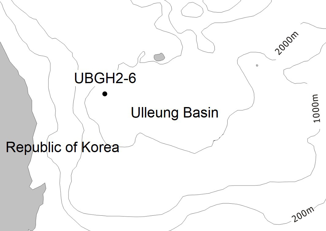
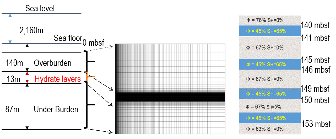
We briefly restate the descriptions of UBGH2-6 in the Ulleung Basin and its numerical domain (Yoon et al., 2021). UBGH2-6 is placed in the deep sea floor under the East Sea, South Korea, as shown in Fig. 1. The depth of water is about 2.1 km, and there are alternating hydrate-bearing sand and mud layers from 140 mbsf and 153 mbsf, which yields the thickness of 13 m. This geological model was constructed from the logging and core data, based on the UBGH2 expedition Bahk et al. (2013); Lee et al. (2013b); Kim et al. (2013); Lee et al. (2013a), Fig. 2 shows the domain of spatial discretization, taking the two-dimensional (2D) axisymmetric domain. The domain size is 250 m × 220 m in the r-(radial) and z-(downward) directions, respectively. Non-uniform gridblocks (160 × 140), refining the hydrate layers and the wellbore region, was used.
Forward simulation
We employed TOUGH+Hydrate code to solve non-isothermal multiphase multicomponent transport problems in porous media associated with gas hydrate deposits (Moridis et al., 2008). The initial pressures at the top (20 mbsf) and bottom (240 mbsf) are 23.1 MPa and 24.6 MPa, respectively, and the initial temperatures at the top and bottom are 6.4°C and 18.6°C, respectively. We applied no flow boundary conditions of multiphase flow and heat flow. The initial porosity and hydrate saturation are shown in Table 1. For all the layers, rock compressibility is 10-8Pa-1, and heat conductivity under desaturated conditions is 1.0 W/m/°C. The other parameters for simulation can be found in the previous studies (Moridis et al., 2013; Yoon et al., 2021).
Table 1.
Rock properties
| Layer type (SH = 0) | Permeability (mD) | Porosity | Rock grain density (kg/m3) |
| Overburden | 0.02 | 0.76 | 2750 |
| Sand interlayer | 500.0 | 0.45 | 2650 |
| Mud interlayer | 0.14 | 0.67 | 2750 |
| Underburden | 0.02 | 0.63 | 2750 |
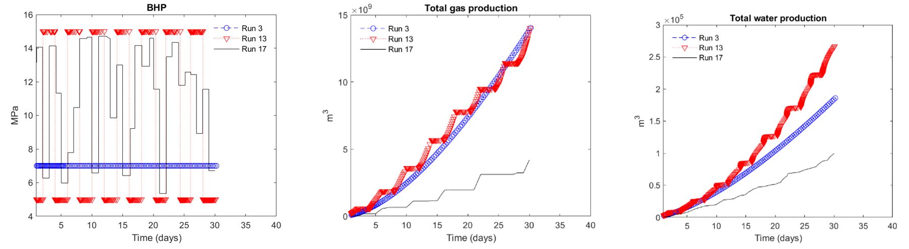
We generated a dataset under various depressurization scenarios for 30 day production. Specifically, we had simulation runs with different bottom hole pressures (BHPs) as follows (Table 2). We used 5 MPa and 15 MPa as minimum and maximum limits of BHP, respectively. BHP below 5 MPa can cause substantial subsidence and wellbore slip, while BHP above 15 MPa might not meet gas production for economic feasibility (Yoon et al., 2021). Fig. 3 shows some simulation results of gas and water production as well as the corresponding BHPs. Run 3 and Run 13 yield higher total production of gas and water than Run 17 because their average pressures are lower. Specifically, in Run 13, gas and water production does not occur at a BHP of 15 MPa, as the pressure is too high.
Table 2.
Depressurization scenarios
| Runs 1‒11: | Constant BHP: 5, 6, 7, …, 15 MPa |
| Runs 12‒16: |
Cyclic BHP between 5 and 15 MPa Frequency: 1, 2, 4, 8, and 16 days |
| Run 17‒24: | Random daily BHP control ranging from 5 to 15 MPa |
The random BHP cases take more than simulation time that the other cases due to frequent changes of BHPs. When BHP is changed, the time step size becomes very small to capture sudden changes of physical processes induced by the changed BHP. Thus, it might not be practical to use this forward simulation during real-time operation, but surrogate models based on many prior forward simulations can provide reliable solutions in real time.
Deep Learning Modeling
The raw dataset consists of well production pressure (i.e., BHP) and flow-rate time series obtained from multiple simulation runs, where each run corresponded to a unique case identifier. Target variables containing flow rates were integrated over time using the trapezoidal approach in discrete form, such that cumulative gas and water production were computed incrementally across timesteps. For the feature data, BHP values were interpolated onto a standardized time grid. The interpolation grid combined a finer resolution in the early-time period (10-2 days to 1 day, ∆t = 0.05 days) with a coarser resolution thereafter (1 day to 30 days, ∆t = 0.5 days), in order to capture transient behavior more accurately during the initial production phase. The same interpolation schedule was applied to the target data to ensure strict temporal alignment between features (inputs) and targets (outputs).
The partitioning of the data into training, validation, and testing subsets was performed at the case level to prevent temporal leakage between sets. Two partitioning scenarios were considered. In the basic case, a total of 16 simulation cases were available, of which 10 (62.50%) were used for training, three (18.75%) for validation, and three (18.75%) for testing. The validation set consisted of cases 7, 13, and 14 (throughout this document, the terms Run and Case are used interchangeably), while the testing set consisted of cases 2, 8, and 15; the remaining 10 cases were used for training. In the expanded case, the dataset comprised 24 simulation cases. In this configuration, 16 cases (66.67%) were used for training, four (16.67%) for validation, and four (16.67%) for testing. The validation set consisted of cases 7, 13, 14, and 23, and the testing set consisted of cases 2, 8, 15, and 20; the remaining 16 cases were used for training. In both scenarios, the split ensured that all time steps from a given case were contained entirely within a single subset, preserving the independence of the evaluation and validation data. Table 3 summarizes the distribution of cases across subsets. Feature and target matrices were converted to NumPy arrays and normalized separately using MinMaxScaler from the scikit-learn library (Pedregosa et al., 2011). The feature scaler was fit on the training set and applied consistently to validation and testing sets. Target scaling was performed in the same manner.
The proposed regression framework is based on a LSTM neural network architecture designed to capture temporal dependencies in sequential data. The original dataset was divided into training, validation, and testing subsets. To make the data compatible with the LSTM layers, the input features were reshaped into a three-dimensional format (N, T, V ), where N represents the number of samples—matching the Case Count presented for each dataset in Table 3—T denotes the number of time steps, fixed at 80, and V represents the number of feature variables, here kept at one.
Table 3.
Distribution of simulation cases across training, validation, and testing subsets for basic and expanded scenarios
The LSTM model was developed using the Keras deep learning library within the TensorFlow framework (Abadi et al., 2016), with hyperparameter optimization conducted through Keras Tuner. The architecture begins with an input layer matching the specified sequence length (timesteps) and feature dimension, followed by a normalization layer to standardize input features. The number of stacked LSTM layers is treated as a hyperparameter, tunable between two and four layers. Within each layer, the number of hidden units is selected from the set {16, 32, 64, 128, 256}. The activation function for recurrent units is chosen between hyperbolic tangent (tanh) and rectified linear unit (ReLU). L2 kernel regularization is applied to each recurrent layer, with the regularization coefficient drawn from {10-4, 10-3, 10-2}. Between LSTM layers, a Leaky ReLU activation function is included with slope parameter α selected from {0.0, 0.1, 0.2, 0.3, 0.4, 0.5}. Dropout regularization is optionally applied after intermediate layers, with a dropout rate searched over {0.0, 0.1, 0.2, 0.3, 0.4, 0.5} to help prevent overfitting and improve generalization. Batch normalization may also be incorporated based on tuning settings. The output layer is a single dense neuron producing one scalar regression value modeled with L2 weight regularization, where the coefficient is also a tunable hyperparameter. Hyperparameter tuning employed random search over 500 trials within this search space, which also included the optimizer choice (either Adam or AdamW), learning rate values {10-5, 10-4, 10-3}, batch sizes from 2 to 9, and, for AdamW, the weight decay rate selected from {10-5, 10-4, 10-3}.
Each candidate model identified by the tuner was trained for a maximum of 200 epochs, with an early stopping criterion applied to the validation loss. Training was stopped if the validation loss did not improve for 20 consecutive epochs, and the weights corresponding to the best-performing epoch were restored. The mean squared error (MSE) was used as both the loss function for optimization and the primary evaluation metric. Following hyperparameter optimization, the best-performing configuration was evaluated on the independent test set.
Sensitivity Analysis - Model Architecture
Shapley Additive Explanations (SHAP) is a powerful method for interpreting complex machine learning models by quantifying each input feature’s contribution to the model’s predictions (Lundberg and Lee, 2017). Rooted in cooperative game theory, SHAP assigns Shapley values that fairly distribute the prediction output among features, reflecting their average marginal contributions across all possible feature subsets. This framework enables consistent and theoretically sound interpretation of model behavior both globally and locally. Formally, the SHAP value for a feature is defined as
,
where is the set of all features, is any subset of features not containing , and represents the model’s prediction using the features in subset . The Shapley value thus captures the average marginal contribution of feature over all feature subsets.
Unlike permutation feature importance, which measures the decrease in overall model performance when a feature’s values are randomly shuffled across the dataset (thereby providing a global importance measure without directionality) (Pedregosa et al., 2011; Baek et al., 2023), SHAP offers detailed, directional explanations of how each feature’s value influences individual predictions. This local interpretability allows understanding both the magnitude and direction of feature effects, making SHAP particularly valuable for analyzing complex models. In this study, SHAP analysis was applied to a RandomForestRe-gressor with 500 estimators trained on various LSTM architecture hyperparameters to elucidate the relative influence of these hyperparameters on model performance.
Results & Discussion
Models were developed with two different datasets (i.e., basic and expanded as detailed in Table 3) to predict cumulative production volumes of water and gas over time based on BHP profiles. To identify optimal architectures for time series forecasting, multiple LSTM-based models were trained using hyperparameter tuning. Table 4 summarizes the four best-performing models identified during this tuning process, highlighting the selected hyperparameters including the number of LSTM layers, activa-tion functions, layer sizes, regularization techniques, optimizer types, learning rates, weight decay rates, and batch sizes. These optimized configurations reflect the tailored model designs necessary to effectively capture the dynamics in each dataset and production scenario. While training time and inference latency were not systematically tracked due to early stopping and hyperparameter tuning variability, retraining with the finalized model was efficient, and inference—i.e., prediction—was effectively instantaneous on a personal laptop.
Table 4.
Optimized hyperparameters for four models predicting cumulative water and gas-production volumes with basic and expanded datasets
Fig. 4 shows unit plots comparing true values (x-axis) and predicted values (y-axis) from each model for the testing datasets under scaled regimes. Unit plots, which scatter model predictions against true observed values, provide an immediate visual assessment of predictive performance. When points fall along the 1:1 diagonal (as denoted with a red dash line), it indicates excellent agreement between the model’s output and ground-truth data, whereas deviations from this line highlight the extent and direction of any prediction errors. This visualization allows for effective identification of systematic biases, the range of errors across the dataset, and potential outliers. Panels (a) and (b) display results for cumulative water production volume using the basic and expanded datasets, respectively, while panels (c) and (d) correspond to cumulative gas production volume with the basic and expanded datasets. The error metrics presented in Table 5 provide a quantitative evaluation of the predictive performance for cumulative water and gas production volumes using both the basic and expanded datasets.
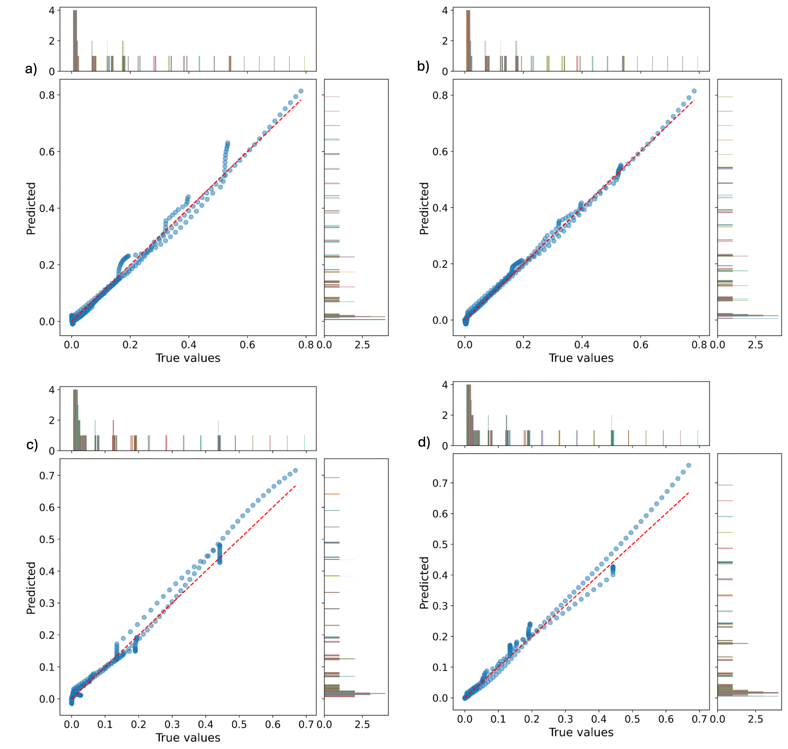
Fig. 4.
Unit plots comparing actual values (x-axis) and predicted values (y-axis) with corresponding histograms for test datasets under scaled data regime. (a) Cumulative water-production volume based on basic dataset, (b) cumulative water-production volume based on expanded dataset, (c) cumulative gas-production volume based on basic dataset, and (d) cumulative gas-production volume based on expanded dataset.
For cumulative water production, both datasets achieved exceptionally high R2 values—0.9792 for the basic dataset and an improved 0.9876 for the expanded dataset—demonstrating that the model reliably captures the underlying production trends. The marginal improvement with the expanded dataset suggests that the additional data or features contribute positively, albeit modestly, to the model’s prediction power. In contrast, for cumulative gas production, the R2 values are comparatively lower, with 0.7483 for the basic dataset and a substantially higher 0.9178 for the expanded dataset. This notable increase reinforces the value of the expanded dataset in enhancing model performance for gas production prediction, possibly due to increased data variability captured. Overall, these R2 values reflect strong predictive capabilities, with especially pronounced gains observed when utilizing the expanded datasets. This underscores the importance of data richness in improving model robustness and accuracy across both production types.
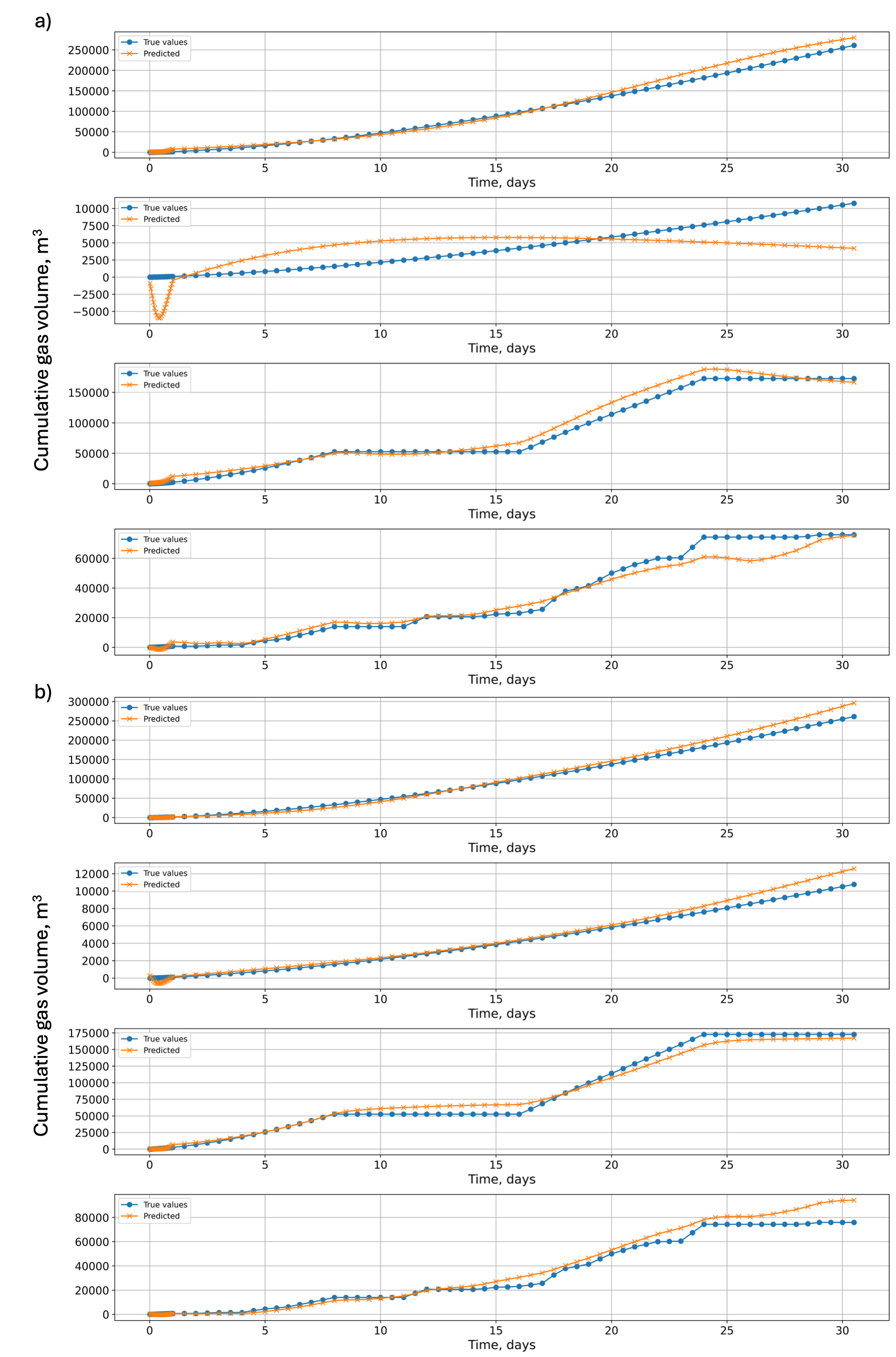
Fig. 5 presents the time-series predictions of cumulative water production volume on the testing dataset, plotted alongside true values in their original scale. Panel (a) shows predictions using the basic dataset, whereas panel (b) displays results for the expanded dataset. Both panels share the same ground-truth curve, enabling a direct, side-by-side comparison of model performance. Fig. 6 shows analogous results for cumulative gas production volume on the testing dataset. Again, panel (a) illustrates model predictions against actual values using the basic dataset, while panel (b) presents results for the expanded dataset. Note that the basic dataset does not include varying BHP scenarios, whereas the expanded dataset does. For a consistent comparison, the test data from the expanded dataset—comprising case IDs 8, 15, 2, and 21—was used to evaluate both models.
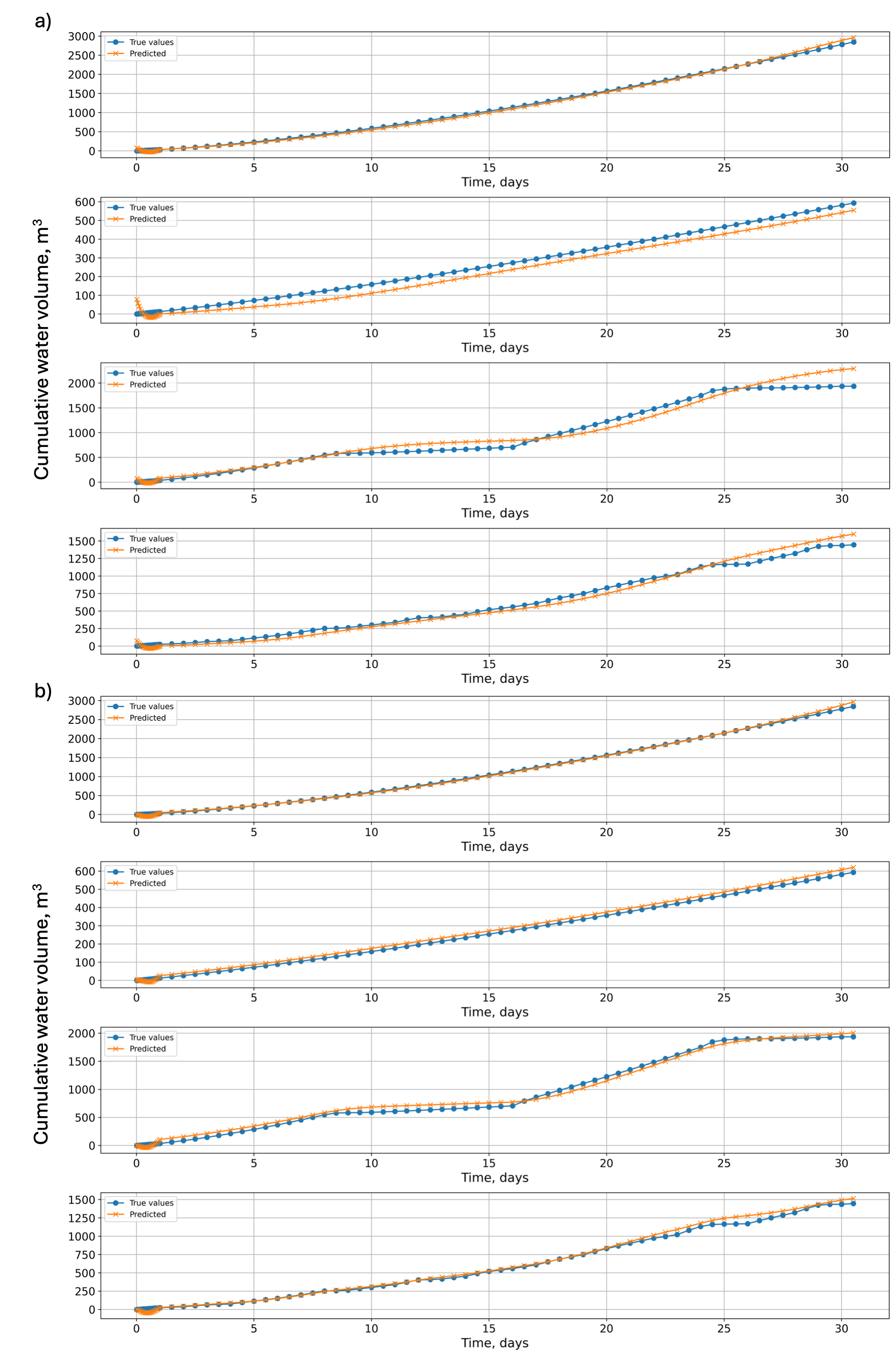
The error metrics presented in Table 5 summarize the performance of the models predicting cumulative water and gas production volumes using both basic and expanded datasets. For water production, the models demonstrate excellent predictive accuracy, with high R2 values reflecting a very high level of fit as discussed above. Correspondingly, the mean square error (MSE) and mean absolute error (MAE) values are low, further confirming the precision of the water production forecasts. The improvement by using more dataset (i.e., expanded dataset) is not noticeable.
Table 5.
Error metrics (R2, MSE, and MAE) for cumulative water and gas-production volume predictions using two datasets
| Metric | Water | Gas | |||
| Basic | Expanded | Basic | Expanded | ||
| R2 | 0.9792 | 0.9876 | 0.7483 | 0.9178 | |
| MSE | 3.8472 × 10⁻⁴ | 2.6331 × 10⁻⁴ | 4.1745 × 10⁻⁴ | 3.1732 × 10⁻⁴ | |
| MAE | 1.4029 × 10⁻² | 1.1685 × 10⁻² | 1.3431 × 10⁻² | 1.0638 × 10⁻² | |
In contrast, predictions for gas production show more variation in performance between the datasets. As observed above with R2, the model trained on the basic dataset achieves a moderate R2, which substantially improves when trained on the expanded dataset. The reduction in both MSE and MAE values for the expanded dataset corroborates this improved predictive accuracy. Predicting gas production is inherently more challenging due to its discontinuous nature—the model must predict the onset time of gas production—as well as the gas phase’s sensitivity to pressure conditions, given its compressibility and higher nonlinearity. For the discontinuous gas production, the problem can be decomposed into two subproblems: predicting the timing of gas production onset and forecasting production thereafter (see Baek et al., 2023; Nagao et al., 2024).
Notably, although the basic models for both phases were not trained on varying BHP scenarios, their predictions for such cases (e.g., Case 21 in Figs. 5 and 6) remain comparably accurate (water: R2 = 0.984; gas: R2 = 0.964). This robustness may arise because cumulative production volumes are less sensitive to fluctuating operational conditions than instantaneous production rates. Overall, the metrics reveal that while both models perform well, the use of expanded datasets consistently enhances prediction accuracy, particularly for the more challenging gas production volume predictions.
The SHAP summary plots in Fig. 7 illustrate the distribution of individual feature (or hyperparameter) impacts on model predictions for two distinct targets: cumulative water production volume (panel a) and cumulative gas production volume (panel b). For the analysis, models trained with expanded dataset were used. In both plots, each point corresponds to a specific hyperparameter setting, with horizontal placement reflecting the magnitude and direction of the feature’s contribution to the predicted output. The features are vertically ordered by their global importance, and the color gradient from blue (low) to red (high) denotes the feature value spectrum. For categorical features, encoding follows: use batch norm (1 = use, 0 = not use), lstm activation (1 = tanh, 0 = relu), and optimizer (1 = AdamW, 0 = Adam).
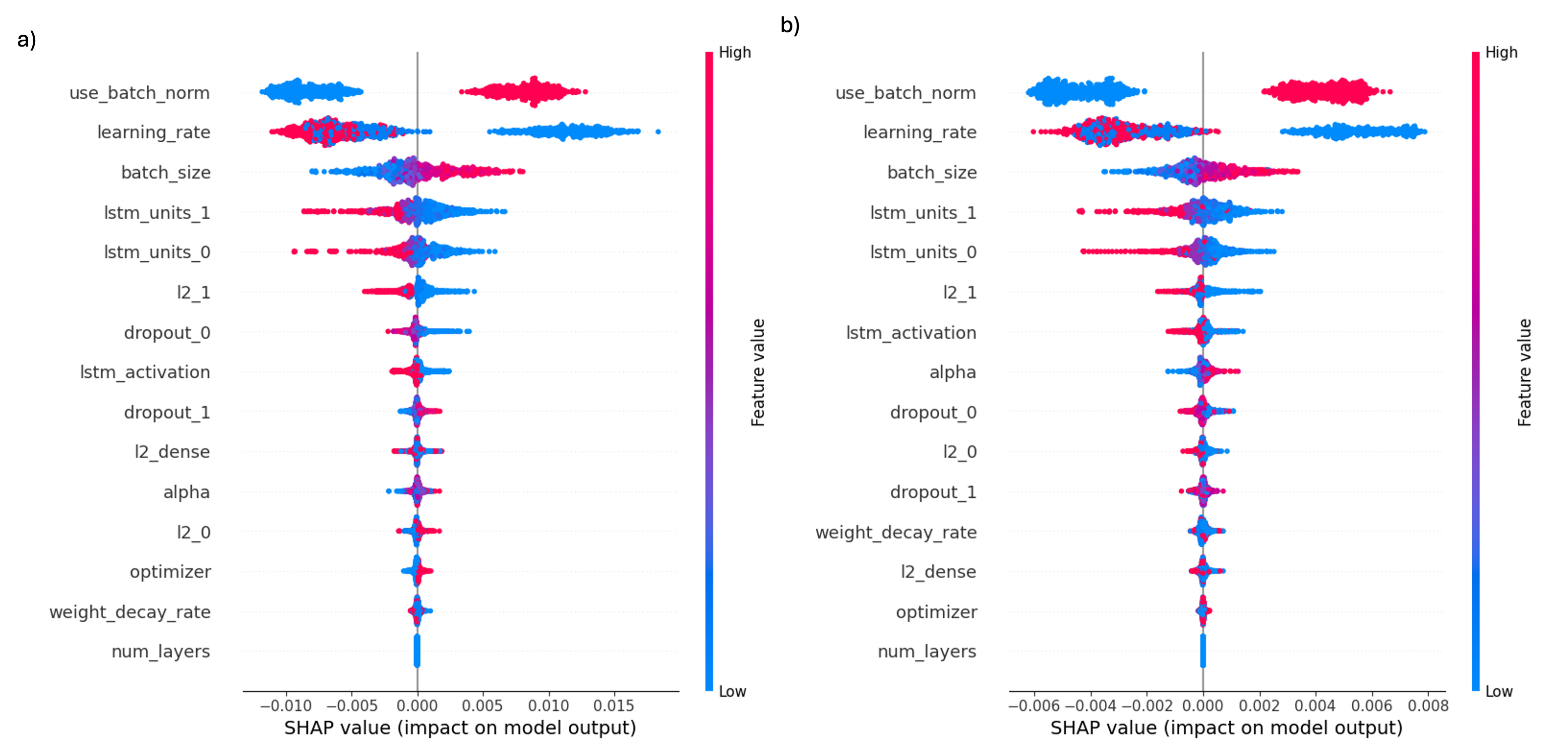
Fig. 7.
SHAP summary plots showing effects of LSTM hyperparameters on model predictions. (a) Cumulative water-production volume; (b) cumulative gas-production volume. X-axis (SHAP value) indicates effect of each hyperparameter on model output, with positive and negative values showing direction and magnitude of effect. Color bar (Feature value) represents actual value of each hyperparameter for corresponding data point, where red and blue indicate higher and lower values, respectively.
For cumulative water production volume (panel a), the binary feature use batch norm demonstrates a strong positive influence; higher values (True) consistently associate with increased SHAP values, confirming the beneficial role of batch normalization in improving predictions. Data that benefits most from batch normalization often has high variability or changing distributions. Batch normalization addresses this by stabilizing feature distributions during training, mitigating the internal covariate shift that occurs when input statistics change between layers (Ioffe and Szegedy, 2015). This leads to smoother and faster convergence, particularly in deep networks with layered features spanning multiple scales (Santurkar et al., 2019). Furthermore, batch normalization acts as a regularizer, helping models trained on noisy or outlier-prone data generalize better by reducing training instabilities and preventing overfitting (Luo et al., 2019). The learning rate also exhibits a clear trend where lower rates (blue) correspond to higher positive SHAP values, indicating that smaller learning rates favor better model performance. By allowing finer and more precise weight updates, lower learning rates diminish the risk of overshooting optimal minima, thereby fostering stable training and robust generalization (Bousquet and Elisseeff, 2002). Data exhibiting high noise, complex nonlinear relationships, or rugged loss landscapes with multiple narrow minima particularly benefit from reduced learning rates, as this setting helps navigate irregular optimization surfaces by mitigating unstable training behaviors (Goodfellow et al., 2016). Other hyperparameters such as batch size and LSTM layer sizes (lstm units 0, lstm units 1) show distinct directional impacts, while most regularization parameters and optimizer type contribute minimally.
The cumulative gas production volume (panel b) exhibits broadly similar feature importance patterns but with subtler magnitudes. use batch norm and learning rate remain primary influencers, though their SHAP value ranges are more compressed, suggesting a somewhat weaker but consistent effect on gas production predictions. The order of importance in features like batch size and lstm units 1 also aligns with the water production model, reinforcing the consistency of these hyperparameters across production metrics. Some additional features such as lstm activation and alpha appear with modest impact on gas volume compared to water volume.
Despite the observed trends, caution is warranted in overinterpreting directional guidance from these plots alone for hyperparameter selection, as extreme settings risk overfitting or underfitting. Overall, this SHAP analysis provides an interpretable, comparative assessment of model architecture influences on regression modeling of both water and gas production volumes, offering valuable guidance for data-driven hyperparameter tuning.
Conclusion
Numerical simulations of gas and water production at UBGH2-6 over a 30-day period were conducted using TOUGH+Hydrate as the forward simulator for gas hydrate flow problems, under both constant and varying BHP production conditions. These simulations required substantial computational time, especially when the BHP was frequently adjusted. To overcome this limitation, surrogate models based on the simulation outputs were developed to provide efficient alternatives to the forward simulator.
LSTM-based surrogate models were developed to predict cumulative production volumes of water and gas using BHP signals. Two models were developed for each phase based on the basic and expanded datasets, with the larger dataset contributing to improved prediction accuracy. Despite the limited dataset and single input feature (i.e., BHP), water production predictions demonstrated high accuracy (R2 ≈ 0.9792−0.9876) for both datasets. Gas production predictions were less accurate probably due to the nature of the fluid phase, but the improvement from (R2) 0.7483 to 0.91 when using the expanded dataset was substantial. As more diverse data are used, the performance of the LSTM improves, highlighting the importance of data size and quality. This indicates potential for further enhancement through incorporation of additional inputs, such as temperature signals.
Sensitivity analysis of the model architecture using SHAP values provided insights into the influential components affecting prediction performance. For both water and gas predictions, batch normalization usage, learning rate, and batch size consistently ranked as the top influences, despite differing prediction targets. While these findings are problem-specific, they offer a valuable starting point for future extended modeling and applications.
